About this text
This revision of the book was last updated on December 8, 2025.
|
This is an old revision of the Remix. The current revision can be viewed here. |
CAUTION - CHAPTER UNDER CONSTRUCTION!
NOTICE: If you are NOT enrolled in the CSC 230 course that I teach at SFSU, you probably are looking for the “public version” of the book, which I only update between semesters. The version you are looking at now is the “CSC230 version” of the book, which I will be updating throughout the semester.
This chapter was last updated on June 19, 2025.
This work, "Discrete Math - The MKD Remix" by Mark Kelly Davis, is adapted from “Discrete Math” by Mohamed Jamaloodeen, Kathy Pinzon, Daniel Pragel, Joshua Roberts, and Sebastien Siva. “Discrete Math” is used under CC BY-NC 4.0. All files for “Discrete Math” are available at its associated GitHub repository.
This work, "Discrete Math - The MKD Remix", is licensed under CC BY-NC 4.0 by Mark Kelly Davis.
|
If you were a student in my course during the Spring 2024 semester, the version of the book you used can be found here. If you were a student in one of my courses during the Fall 2024 semester, the version of the book you used can be found here. If you were a student in one of my courses during the Spring 2025 semester, the version of the book you used can be found here. If you were a student in one of my courses during the Fall 2025 semester, the version of the book you used can be found here. |
How does the Remix differ from the original work?
The remixer’s goal is to adapt the original “Discrete Math” to create an OER textbook for a one-semester Discrete Mathematics/Discrete Structures course for Computer Science students who have some experience coding in Java, Python, or another high-level programming language, and have completed an Algebra Ⅱ-level (or equivalent) mathematics course. The Remix is a work-in-progress that will continue to evolve over time toward this goal.
Use of materials from the Discrete Mathematics Project
The Remix is designed to work with the activity-based lesson materials developed by the Discrete Mathematics Project (DMP.) See the Appendix: For Instructors for information on how the remixer uses these lessons with the text.
Alignment To Standards
The remixer’s intent is that the Remix:
-
address topics and learning outcomes listed for
-
ACM/IEEE-CS/AAAI Joint Task Force on Computer Science Curricula "Computer Science Curricula 2023" MSF-Discrete: Discrete Mathematics
-
ACM/IEEE-CS Joint Task Force on Computing Curricula "Computer Science Curricula 2013" Discrete Structures (DS) but omitting the DS/Discrete Probability topics and learning outcomes.
Note: ACM CCECC "Computer Science Curricular Guidance for Associate-Degree Transfer Programs with Infused Cybersecurity" Discrete Structures Knowledge Area (DS) is a list of learning outcomes and assessment rubrics that does not specify topics, so the remixer preferred the 2013 document to that June 2017 update. -
California Community Colleges (CCC) C-ID Math 152: Discrete Structures content areas Ⅰ through Ⅴ, omitting area Ⅵ. Discrete Probability.
Note that the content listed for C-ID Math 152: Discrete Structures is identical to the topics listed for ACM/IEEE-CS CS2008 Review Taskforce "Computer Science Curriculum 2008: An Interim Revision of CS 2001" Discrete Structures (DS). -
additional topics from the ACM CCECC Software Engineering curriculum 2005 Discrete Structures Mathematics course.
-
Other Considerations in the Remix
In addition to using activity based lessons and aligning to the standards, the Remix aims to:
-
use terminology, definitions, notation, and symbols that align with commonly-used textbooks such as Kenneth H. Rosen’s Discrete Mathematics and Its Applications, 8th Edition.
-
give students the opportunity to learn new content based on what they already know then to move toward building a more formal understanding of the content (e.g., pointing out that the set of odd integers and the set of even integers are the two equivalence classes of an equivalence relation, , and that the rules for adding and multiplying "odds" and "evens" is an example of modular arithmetic.)
-
organize the content in "chunks" for ease of reading and digestion of new ideas
-
refer to original sources (e.g., Pascal’s handwritten triangle as well as earlier non-European references to and uses of the number triangle.)
If you are looking for an OER textbook for a Discrete Mathematics course intended primarily for Mathematics majors (e.g., one that does not include topics like analysis of algorithms and binary tree traversal), there are many suitable ones that exist. For example, see Oscar Levin’s Discrete Mathematics: An Open Introduction, 4th edition.
About the use of Python in the Remix
The Remix is intended for a course that does not require programming. Python is not part of the course content.
The original “Discrete Math” uses Python code samples throughout the textbook and includes "Introduction to Python" as its 3rd chapter. The Remix repurposes this content: Code samples in the Remix are used as "pseudocode that can run on a computer," with coding that uses "just enough Python" to illustrate important abstract ideas and concepts. Most of the existing Python examples were altered, and many new Python examples were introduced throughout the Remix. Note that, in order to illustrate concepts and ideas in the style of pseudocode, much of the Python code shown in the Remix avoids using built-in functions and often uses less efficient data structures and algorithms! For example, in the chapter "Algorithms & Big-O", code samples for sorting and searching avoid using built-in Python functions in order to illustrate all steps needed by the algorithm. In many cases, a comment can be found near a non-optimal code example that explains or illustrates a more Pythonic way of coding.
Partial list of changes made (or to be made) to the Remix.
-
Terminology, definitions, notation and symbols were changed throughout the Remix to align with other commonly-used textbooks. For example, the Remix defines the set of natural numbers \(\mathbb{N}\) to include the integer 0 as an element; this definition is very common and is in fact a "standard" that appears in International Standard ISO 80000-2:2019, Quantities and units — Part 2: Mathematics.
-
In the chapter "Introducing Discrete Mathematics," informal definitions of foundational mathematical ideas needed in the course are introduced. This is done so that learners can see what they do (or do not) already know and create the necessary basis to learn the course content. In addition, a new Appendix, "On-Demand Math Resources" was written which includes material that learners can refer to as needed.
-
The original chapter "Introduction to Python" was moved to the appendices.
-
The original chapter "Counting" was split into two chapters, "Counting: Arithmetic Techniques" and "Counting: Permutations And Combinations". The first of these chapters is placed near the beginning of the book, but the second is place much later, after sequences and recurrence relations have been discussed.
-
The order of the chapters "Set Theory" and "Logic" was swapped. New material was inserted into each of the two chapters.
-
A new chapter, "Proofs: Basic Techniques," was written and inserted after "Logic."
-
The chapter "Number Bases" is based on the original chapter "Number Theory," but the content on divisibility, congruence, and modular arithmetic was moved into the remixed chapters "Introducing Discrete Mathematics" and "Relations."
-
The chapter "Sequences and Recursion" is based on the original chapter "Sequences, Recursive Definitions, and Induction," which was split into two new chapters, "Sequences and Recursion" and "Proofs: Mathematical Induction." "Sequences and Recursion" appears before and as a lead-in to "Functions" since sequences are a special case of functions and recursion is often used to define functions.
-
The chapter "Functions" was moved to its new position, several chapters after "Set Theory." This was done for the following reasons:
-
The learner is expected to have a basic working understanding, from previous classes, of the one-to-one correspondence concept: A unique pairing of each element in one set with elements in another set.
-
The learner is expected also to have a basic working understanding of the function concept: A rule/mapping/association that takes certain objects as inputs and assigns each such input to exactly one output object.
-
It is likely that the learner has some ability to work with function notation and operations such as composition and inversion of functions from previous mathematics courses.
-
The remixer felt that a precise, formal definition of function, as well as properties such as injectivity and surjectivity, could be delayed until after learners had used their previous knowledge of functions.
-
-
A new chapter, "Relations," was written to include topics listed in the ACM/IEEE-CS/AAAI and CCC C-ID courses but absent from the original work, and was inserted after "Functions". This chapter also includes some of the content on divisibility, congruence, and modular arithmetic from the "Number Theory" chapter of the original work.
-
The chapter "Proofs: Mathematical Induction" is based in part on the original chapter "Sequences, Recursive Definitions, and Induction," but the content of this chapter was heavily rewritten and new content was inserted. This chapter was placed immediately before the chapters "Rates of Growth of Functions" and "Algorithms and Their Analysis" so that mathematical induction can be viewed as a way of validating algorithms rather than as just another more complicated proof technique.
-
The order of the chapters "Algorithms" and "Growth of Functions" was swapped, then the title "Growth of Functions" was changed to "Rates of Growth of Functions" and the title "Algorithms" was changed to "Algorithms and Their Analysis." New content was inserted into each of the chapters and existing content was revised.
Note that algorithms and their analysis are not mentioned explicitly as topics to be included in the ACM/IEEE-CS/AAAI and CCC C-ID courses, but these topics fit naturally as a motivation to learn much of the other content of the Remix.
-
The original chapter "Graph Theory" was split into two chapters, "Graphs" and "Trees". Additional content will be introduced into each of the new chapters.
1. Introducing Discrete Mathematics
NOTICE: If you are NOT enrolled in the CSC 230 course that I teach at SFSU, you probably are looking for the “public version” of the book, which I only update between semesters. The version you are looking at now is the “CSC230 version” of the book, which I will be updating throughout the semester.
This chapter was last updated on July 9, 2025.
Welcome to the Remix! I hope this textbook provides you an opportunity for a stimulating and intellectually enjoyable learning experience.
Mathematics is one of human civilization’s greatest tools: It involves pattern noticing, collecting, comparing, counting, generalizing, formalizing, and abstracting. The development of mathematics is a continuing work that spans at least 5,000 years and many different peoples and cultures. This development will continue long after you and I are gone - never forget that we are living during an era that will be someone else’s Ancient History!
1.1. What is "Discrete Mathematics"?
There seems to be no universally agreed-upon definition of "discrete mathematics," but I will describe to you my understanding of what the phrase "discrete mathematics" means.
Discrete mathematics is the mathematics people use to study and understand structures that are built from individual objects in a way that the individual objects can still be treated as separate from one another within the structure. In such a structure, the individual objects can be put into categories and counted; it makes sense to ask questions like "What is the next object in the structure after this one?" or "Which other objects are the closest to this one?" (where "closest" could refer to physical distance or could mean most similar in color or size) or "How many objects in the structure have a certain property?" Discrete mathematics is a collection of tools that can be used to answer these kind of questions.
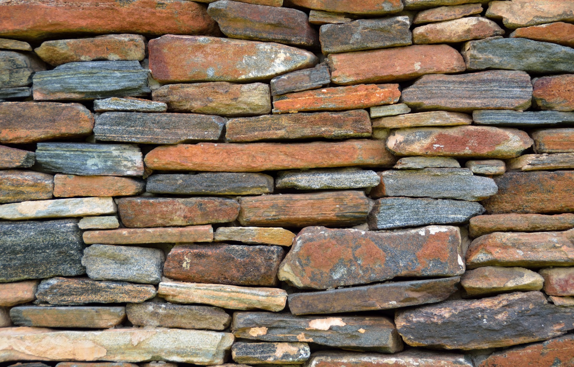
As an example, consider a wall, a structure built from individual stones and bricks, part of which is shown in the image.
The
individual
objects in the structure are
the stones and bricks. You can still identify individual objects even though they were combined to build the larger structure, and can classify
an
individual object
by type (either stone or brick) or by color or by the how close to the top of the wall the object
is. You can try to count the total number of individual objects, and you can count the number of individual objects that are next to any one object you choose. The wall is a (non-mathematical) example of a discrete structure.
Image credit: "Vintage Stone And Brick Wall" by Paul Brennan. The image is dedicated to the public domain under CC0.
Here are two more examples of discrete structures.
-
A family of humans can be treated as a discrete structure.
The humans in a family are seen as individuals who can be distinguished from one another. Questions like "Which humans are siblings of this human?" and "Which humans are parents of this human?" and "How many children does this human have?" make sense. -
The set of integers, in the usual order, as represented on a number line is a discrete structure.
It makes sense to ask questions like "What is the next integer after -2?" or "What are the integers that are closest to -2?" for this structure.
Notice that in these examples, the individual objects are of a different nature than the entire structure: Individual bricks and stones aren’t considered a wall, individual humans aren’t considered a family, and individual integers are not a collection of integers.
So what kind of structure is not discrete?

Consider the water in the glass shown in the image. The water in the glass is a structure, but for most of human history it has not been seen as made up of objects that are of a different nature than the structure. That is, many generations of humans have recognized the difference between a wall and the individual stones and bricks that make up the wall, but likely have perceived water as being made up of… water. This is why humans tend to use measurement of quantities of water, using units such as fluid ounces or milliliters.
In our current era,
we humans understand that the water is built from molecules,
which are of a different nature than the water
"structure,"
but because the molecules are so tiny, numerous, and densely distributed throughout the structure, we humans (except perhaps some scientists and engineers)
still use measurement instead of counting and ignore the individual molecules.
For example, a recipe might call for "8 ounces of water" but never would ask for "7.6 × 1024 molecules of water." Notice that the measurement units used do not correspond in any natural way to individual molecules or groupings of individual molecules (unless, perhaps, you are a scientist or engineer.)
Also, notice that the glass container itself is another structure in which the individual molecules tend to be ignored.
Image credit: "Water Glass" by Peter Griffin. The image is dedicated to the public domain under CC0.
Humans use continuous mathematics like calculus to study a structure that is built from objects that are densely distributed throughout the structure. For such a structure, measurement and approximation is more appropriate than counting.
-
The set of real numbers, in the usual order, as represented on a number line is NOT a discrete structure.
It does NOT makes sense to ask about "the next real number after \(\pi\) on the number line" because if we think c is "the next real number after \(\pi\) on the number line" then we can compute the number \(c_{1} = \frac{c+\pi}{2},\) which is the midpoint of the interval with endpoints \(\pi\) and c, so \(c_{1}\) is closer to \(\pi\) than c is, which means \(c_{1}\) is a better candidate for "the next real number after \(\pi\) on the number line" than c … so the concept "the next real number after \(\pi\) on the number line" does not make sense for this structure as such a number cannot exist! We can just keep computing numbers that get closer and closer to \(\pi\) over and over again. Likewise, "the real numbers that are closest to \(\pi\)" do not exist.
Instead, it makes sense to talk about "the real numbers that differ from \(\pi\) by less than \(\epsilon\)" where \(\epsilon\) is some positive real number (The symbol \(\epsilon\) is the Greek letter "epsilon".) By choosing \(\epsilon\) as small as we like, we can describe the real numbers that are as close to \(\pi\) as needed to use as approximations to \(\pi.\) This is why and how limits are defined and used in courses like precalculus and calculus, subjects that involve the real number line.
Note 1: You could use any other real number instead of \(\pi\) in the discussion above because the argument will still be valid. For example, "the next real number after \(-2\) on the number line" and "the real numbers that are closest to \(-2\) on the number line" do not exist since you can choose numbers that get closer and closer to \(-2\) such as \(-1,\) \(-1.5,\) \(-1.75,\) and so on.
Note 2: The technique used to justify that "the next real number after \(\pi\) on the number line" does not exist is called proof by contradiction and will be discussed along with other techniques in the Proofs: Basic Techniques chapter of this textbook.
Note 3: Is \(\pi\) really on the number line? Click here to view an artist’s explanation about where \(\pi\) lies on the number line. Be warned that some of what this artist says (about history, about \(\pi\) being equal to 3.14) is not correct, but the visualization still may be helpful to you.
Note 4: FYI, the set of real numbers is called the continuum in advanced mathematics courses.
1.2. To The Student: Some Things To Know Before You Begin
Here are some things to orient you.
1.2.1. How To Use This textbook
The Remix is designed to build on your previous knowledge, and then build new knowledge and understanding by visiting the topics over and over again. In the next subsection, the basis of foundational mathematical ideas are discussed. You are encouraged to read through all of those foundational topics and to work through the Questions and Challenges.
There are two analogies that I, the remixer, like to use here:
-
Think of the course presented in the Remix as a language course.
You will use this language to talk about mathematics and computer science as you continue along your professional path. You cannot master a new language by learning some words or grammar in the first few weeks of a language course and then "forgetting" that content later, but still succeed in the course and master the language to use beyond the course. You need to assume that everything you learn in this textbook will apply later in the textbook and in your later learning. One of the goals of this textbook is to help you build a broad and rich vocabulary in discrete mathematics and a way of thinking that will apply to your future work. -
Think of the course presented in the Remix as exercising at a gym.
You will build your strength and awareness about your abilities by working out. It may be tempting to watch others "demonstrate" how to do certain exercises and then choose not to do them yourself, but you are selling yourself short. A physical trainer usually knows already what they are capable of doing, so it is no compliment if you tell them "Wow, you’re really strong"… the trainer’s goal is to get you to say "Wow, I’m starting to get really strong!"
1.2.2. Foundations
Learning discrete mathematics requires putting together old ideas in new ways and adding new ideas to your mix.
This subsection highlights some of the ideas you will need to work with in order to get the most out of this textbook. Also, you’ll find opportunities here to practice with the built-in tools that are part of the textbook. Some of these ideas may be old for you, but others will probably be new. To use this textbook effectively, you’ll need to be able to work with each of these ideas with relative ease. If a few of these ideas are brand new to you, that is fine: All of these ideas will be discussed again, much more formally and in greater detail, later in the textbook.
I encourage you to read all of the topics discussed below. Don’t skip anything, even if it looks "old" because there may be some new ways of understanding the old ideas that are introduced and that will be used later in the course.
-
A set is an unordered collection of zero or more objects. You can think of a set as a list of the names of the objects included, but we do not care about the order of the names in the list and we do not care if the list contains duplicate names.
An example is the set of the names of the additive primary colors of light which can be written as \[\{ \text{"red"},\,\text{"green"},\,\text{"blue"},\,\text{"red"} \}\] which contains exactly three elements: "blue", "green", and "red." It does not matter that "red" appears twice, and it does not matter that the order of the colors in the list "blue", "green", and "red" is different from the order used in the previous set notation. We could define the same set with any other list that contains the same three elements, for example, \(\{ \text{"green"},\,\text{"red"},\,\text{"blue"} \}.\)
As you will see in the Set Theory chapter, it is common practice to use uppercase English letters to stand for sets; this is similar to how lowercase letters are used as variables or constants in algebra. For example, you could write \[P = \{ \text{"red"},\,\text{"green"},\,\text{"blue"},\,\text{"red"} \}\] which allows you to refer to the set as P instead of needing to read the list of elements every time you want to talk about the set. This is like using the Greek letter π instead of needing to read off the first few digits of the non-repeating decimal expansion 3.14159265359… every time you refer to that number.-
NOTE 1: In mathematics, a set like \(P,\) that is, \(\{ \text{"red"},\,\text{"green"},\,\text{"blue"},\,\text{"red"} \}\) is treated as a constant, so you cannot remove elements or insert new elements once a set has been defined and described. As an example, if you wanted to insert the name "white" into the set, you would need to define a new set \[ C = \{ \text{"red"},\,\text{"green"},\,\text{"blue"},\,\text{"red"},\,\text{"white"} \}\] that contains four elements by appending "white" to the list used to define the old set P.
-
NOTE 2:
-
One way of creating a new set from two other sets is to form the union of the two sets. The union of two sets is formed by joining the sets.
For example, If \(P = \{ \text{"red"},\,\text{"green"},\,\text{"blue"},\,\text{"red"} \}\) and \(T = \{ \text{"yellow"},\,\text{"red"},\,\text{"blue"} \}\), then the union of the two sets is \(\{ \text{"red"},\,\text{"green"},\,\text{"blue"},\,\text{"red"}, \, \text{"yellow"},\,\text{"red"},\,\text{"blue"} \},\) the set that contains the colors that are in at least one of the sets \(P\) and \(T.\) -
Another way of creating a new set from two other sets is to form the intersection of the two sets. The intersection is the meeting of the two sets.
For example, If \(P = \{ \text{"red"},\,\text{"green"},\,\text{"blue"},\,\text{"red"} \}\) and \(T = \{ \text{"yellow"},\,\text{"red"},\,\text{"blue"} \}\), then the intersection of the two sets is \(\{ \text{"red"},\,\text{"blue"} \},\) the set that contains the colors that are in both of the sets \(P\) and \(T.\)
Likewise, if \(S = \{ \text{"yellow"},\,\text{"cyan"},\,\text{"magenta"} \},\) the set of additive secondary colors, then the intersection of \(P\) and \(S\) is the set \(\{ \},\) the set that contains zero elements. We call the set \(\{ \}\) the empty set.
-
-
NOTE 3: We can define a subset of any set by selecting zero or more of the members of the set. For example, \(\{ \text{"green"},\,\text{"blue"} \}\) and \(\{ \text{"green"} \}\) are subsets of \(\{ \text{"red"},\,\text{"green"},\,\text{"blue"},\,\text{"red"} \},\) and so is \(\{ \},\) the empty set.
-
NOTE 4: A set can also be defined by a property instead of a list. This will be explained in the Set Theory chapter.
-
-
A one-to-one correspondence between two sets A and B is a pairing of each member of the set A with exactly one member of set B, and each member of set B with exactly one member of set A.
As a first example, the one-to-one correspondence between the set of uppercase English letters and the set of lowercase English letters is represented in the image. You can choose each letter in the upper row and follow the arrow down to the corresponding lowercase letter that it is paired with.
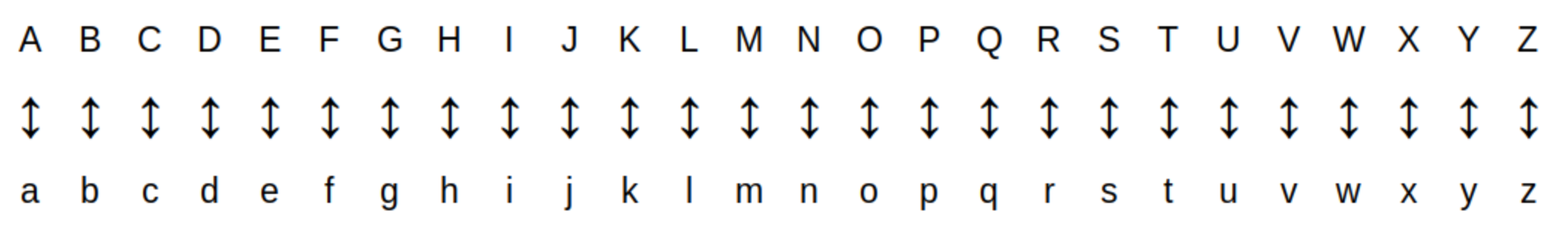
Notice that you could choose any lowercase letter in the image and follow the arrow up to its corresponding uppercase letter. This shows that the one-to-one correspondence
is invertible in the sense that there is a second one-to-one correspondence that can "undo" what the first one-to-one correspondence does.
This is why the arrows in the image point in both directions: It is natural to interpret the arrow as meaning "change case" in either direction.
In fact, the image for the one-to-one correspondence actually represents two functions: The first function is the uppercase-to-lowercase conversion that uses only the down arrows, and the second function lowercase-to-uppercase conversion that uses only the up arrows.
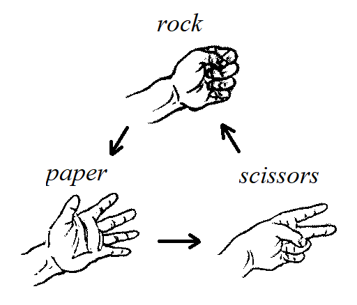
As a second example, consider the game "rock, paper, scissors."
The image represents the one-to-one correspondence that pairs each element of the set \(\{ \text{"rock"},\,\text{"paper"},\,\text{"scissors"} \}\) with the element of the same set that it loses to.
Image credit: Remixer-created derivative of original work "THE_GAME_OF_KEN.(1910)-illustration-_page_315.png". According to Japanese Copyright Law (June 1, 2018 grant) the copyright on the original work has expired and is as such public domain. Also, the original work is in the public domain in the United States because it was published (or registered with the U.S. Copyright Office) before January 1, 1930.
_-_illustration_-_page_315.png)
For this one-to-one correspondence, it makes more sense to use arrows that point in only one direction.
In the image, all the arrows point to the winner, so each arrow can be read as "loses to," for example "rock loses to paper".
Note 1: A one-to-one correspondence between a set and itself is called a permutation. You will see the term "permutation" again, used with a related but different meaning, in the Counting: Permutations and Combinations chapter.
Note 2: "Rock, paper, scissors" is a modern form of a very old game that appears to date back at least 1,800 years to China during the time of the Han dynasty. You can learn more about the history of "rock, paper, scissors" and other intrasitive games at this Wikipedia link. The image used in the Remix is derived from one that appears in a book published in 1910 that describes the Japanese game stone-ken or jan-ken.
-
A natural number is one of the nonnegative integers. The letter \(\mathbb{N}\) denotes the set of natural numbers, that is, \[\mathbb{N} = \{ 0,\,1,\,2,\,3,\,\ldots \}\] where the three dots are used because we cannot write down the entire list of natural numbers.
-
NOTE: We almost always use the base-ten (decimal) place-value system to represent natural numbers, but later in this textbook you will see that there are other number base systems such as the base-two (binary) place-value system, that are useful in some contexts.
-
WARNING: The definition of natural numbers used in this textbook is an ISO standard, but be aware that other textbooks and sources may use the "nonstandard" definition that the natural numbers are the positive integers. In this textbook, the set of natural numbers ALWAYS include zero as well as the positive integers, which is the standard definition.
-
-
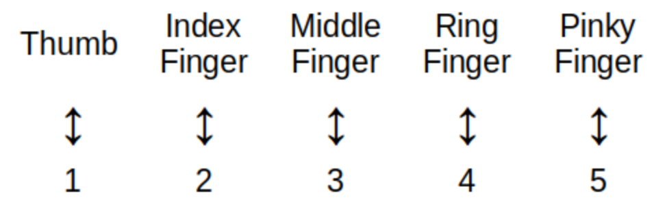
A set is called a finite set if either the set is empty or there is a one-to-one correspondence between the set and \(\{1, 2, \ldots , n \}\) for some positive integer \(n.\) For example, the image represents how a child may "count up to 5" by pairing fingers with the numbers in \(\{1, 2, \ldots , 5 \}.\)
A set that is not a finite set is called an infinite set. Both finite and infinite sets will be discussed in more detail in the Set Theory chapter.
-
You may be surprised to see Counting listed as a topic in a university-level course because you probably learned to count by putting physical objects (like fingers) into a one-to-one correspondence with number words such as "one, two, three, four, five" when you were a young child. That way of counting one by one is fine for small sets, but the counting techniques discussed in this textbook let you count the number of elements in very large finite sets quickly.
The multiplication principle, also called the product rule, is the following statement.
Suppose that we have a procedure that consists of completing two steps, that there are k possible ways to complete the first step, and for each possible way of completing the first step, there are m possible ways to complete the second step. Then there are k⋅m ways to complete the procedure.
As an example, the number of possible strings of 2 characters with the first character being one of the 26 uppercase English letters and second character being one of the 10 Hindu-Arabic numerals is 260 = 26⋅10.
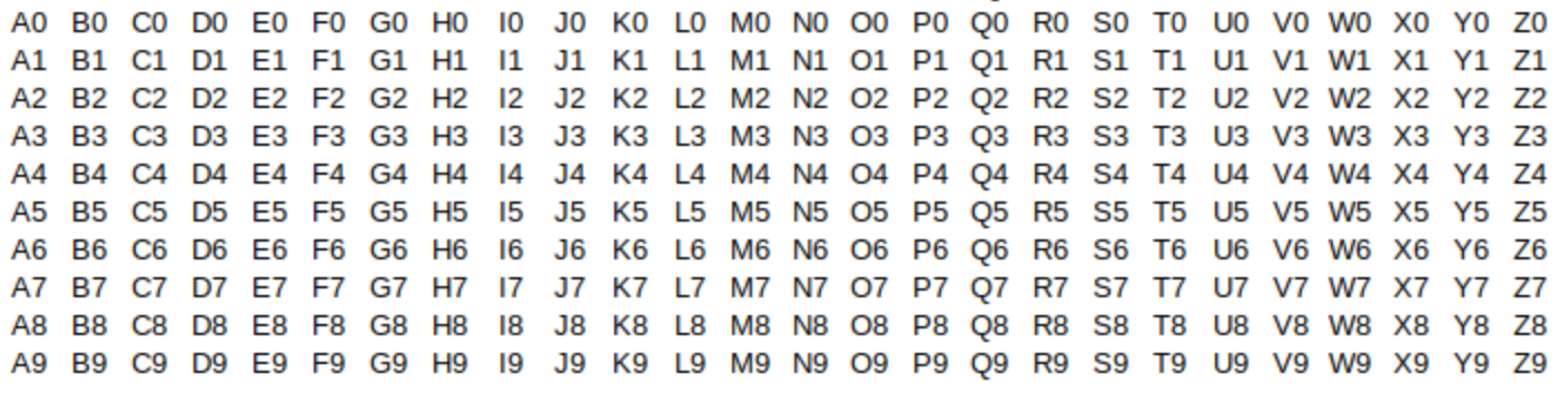
In this case, 26 and 10 are small integers so you can list all possibilities by arranging them in a table as shown in the image. What is important to notice is that this same technique (multiplying k and m) will work for much larger values of k and m, when creating such a table may be either not helpful or impossible.
Click on "Hint," "Another challenge," and "One last challenge" to reveal the hidden text.
With these additional restrictions, how many different possible passenger vehicle license plate numbers can the state create?
-
The Pigeonhole Principle states that if \(n\) is a positive integer and \(n+1\) objects are going to be assigned to \(n\) categories then one of the categories must be assigned at least 2 of the objects. Click here to see a commonly-used photoshopped image that illustrates this principle.
-
A function from set D to set C is a rule that assigns to each element in D (that is, to each input value) exactly one output value from C. We also say each input value is mapped to the output value. A much more formal definition will be given in the Functions chapter of the textbook, but for now it is enough to understand functions in this way.
-
The rule may be represented by a mathematical equation, a verbal description, a table of paired values, a plot of points, … or even code 😎!
-
The set D of all input values is called the domain of the function.
-
The set C that contains the output values is called the codomain of the function.
-
The range of the function is the set that contains only the output values and no other elements. The range is always a subset of the codomain C, but may not contain every element of C. That is, some elements of C may not be outputs for the function. It is often important to distinguish the range from the codomain; this is discussed in detail in the Functions chapter.
-
Here are some examples of functions with their rules, domains, codomains, and ranges.
-
Any one-to-one correspondence between two sets A and B can be viewed as a function \(f\) from A to B.
-
The rule for \(f\) is given by the pairing of elements in A with elements in B.
-
The domain of \(f\) is the set A.
-
The codomain of \(f\) is the set B.
-
The range of \(f\) is the set B, too, because every element in B is paired with an element in A by the one-to-one correspondence.
Notice that the one-to-one correspondence can be used to define another function g from B to A with domain B, codomain A, range A, and rule given by the pairing of elements in B with elements in A. The two functions \(f\) and g are called inverse functions because \(f\) and g "invert" or "undo" each other. Inverse functions will be discussed in more detail in the Functions chapter.
-
-
The floor of x, \(\lfloor x \rfloor,\) and the ceiling of x, \(\lceil x \rceil,\) are two functions defined for all real numbers as follows:
-
\(\lfloor x \rfloor\) is the greatest integer less than or equal to x. For example, \(\lfloor -1.5 \rfloor = -2\) and \(\lfloor 6.3 \rfloor = 6\)
-
\(\lceil x \rceil\) is the least integer less than or equal to x. For example, \(\lceil -1.5 \rceil = -1\) and \(\lceil 6.3 \rceil = 7\)
-
The domain of both the floor and ceiling functions is the set of all real numbers, \(\mathbb{R}.\)
-
The range of both the floor and ceiling functions is the set of all integers, \(\mathbb{Z}\) (NOTE: The German word for "numbers" is Zahlen, which is why the letter \(\mathbb{Z}\) is used for the integers.)
-
The codomain of these two functions can be chosen depending on the context. If we only need to consider output values we could choose the codomain to be the same set as the range, \(\mathbb{Z},\) but if we want to plot these two functions in the xy coordinate plane we would choose the codomain to be the set of real numbers, \(\mathbb{R}.\) This is discussed in the Functions chapter.
The floor and ceiling functions are discussed in more detail in Appendix: Library of Functions.
-
-
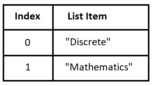
In Python, a list can be used to represent a function with inputs the valid integer indices for the list and outputs the values stored in the list. In an earlier example, we defined list L to be ["Discrete", "Mathematics"] and then evaluated L[0] and L[1] to access the strings stored in the list.
Note for programmers: In reality, the items in the list are references to objects that implement the two strings. That is, the list items are neither the strings nor the objects that implement strings but references to those objects, which are located elsewhere in memory. -
The rule "Return the first character of the input Unicode string."
-
The domain is the set of all strings of length greater than or equal to 1 that contain Unicode characters.
-
The range is the set of all Unicode characters.
-
We would need to decide what the codomain should be in this context: It could be the same as the range, or we could use the larger set of all strings that contain Unicode characters (including the empty string "".)
-
-
\(f(x) = x^{2}\) from the set of real numbers to the set of real numbers.
-
The domain and codomain are both the set of real numbers.
-
The range is the set of nonnegative real numbers.
-
-
\(g(x,\,y) = xy + y\) where x and y are real numbers.
-
The domain is the set of ordered pairs of real numbers.
-
The range is the set of all real numbers. The codomain is the same as the range.
-
-
See the Appendix: Library of Functions for other functions you should be familiar with.
Here is another example.
-
A sequence is a function from the natural numbers, or a subset of the natural numbers, into another set (e.g., the natural numbers, or the real numbers, or a nonnumerical set.) For example, we can define a sequence by the rule \[a_{i} = 2i+1 \text{ for every natural number } i \] which describes the sequence of positive odd integers \(a_{0} = 1,\) \(a_{1} = 3,\) \(a_{2} = 5,\) and so on.
-
NOTE 1: It is common to use i as a variable in sequence notation because i is the initial letter of the word index. This i has nothing to do with the complex number \(\sqrt{-1}.\) Mathematicians recycle and reuse letters!
-
NOTE 2: It is traditional to write the input variable for a sequence as a subscript instead of putting it between parentheses. In the preceding example, \(a_{i} = 2i+1\) has the same meaning as \(a(i) = 2i+1\).
-
NOTE 3: The output values of a sequence are called terms. For example, the 0th term of the sequence is \(a_{0} = 1,\) the 1st term of the sequence is \(a_{1} = 3,\) and so on.
-
-
A finite sequence is a sequence that is defined for only a finite subset of \(\mathbb{N}.\) That is, the set of input \(i\) values that make sense for the sequence is a finite set.
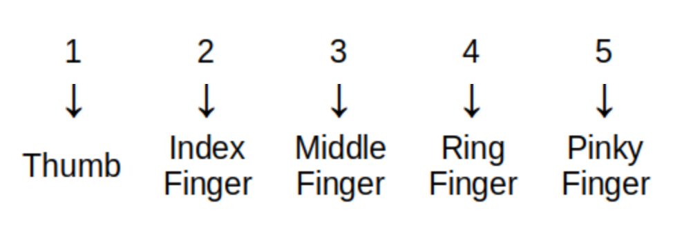
For example, a child counting up to five on the fingers of one hand is defining the sequence called \(\textit{fingers}_{i}\) that is represented by the image.
Technically, the sequence \(\textit{fingers}_{i}\) shown in the image is the inverse of the child’s actual counting sequence. Because the child assigns to each finger "input" exactly one number "output," the arrows would point up from a finger to the corresponding number.
The sequence \(\textit{fingers}_{i}\) can be written, formally, as \begin{equation} \begin{aligned} \textit{fingers}_{1} {} & = \text{"Thumb"} \\ \textit{fingers}_{2} {} & = \text{"Index Finger"} \\ \textit{fingers}_{3} {} & = \text{"Middle Finger"} \\ \textit{fingers}_{4} {} & = \text{"Ring Finger"} \\ \textit{fingers}_{5} {} & = \text{"Pinky Finger"} \\ \end{aligned} \end{equation} but it is much more common to list the terms of the sequence in order: "Thumb," "Index Finger," "Middle Finger," "Ring Finger," "Pinky Finger."
Notice that Java arrays and Python lists are implementations of the mathematical concept of a finite sequence where the domain is the set of \(i\) values \(\{0, 1, \ldots , n \}\) for some natural number \(n.\)
An infinite sequence is a sequence that is not a finite sequence, that is, the there are infinitely many \(i\) values that make sense as inputs for the sequence. For example the sequence \[ \text{isOdd}_{i} = \begin{cases} \text{1} & \text{ if } i \text{ is odd} \\ \text{0} & \text{ if } i \text{ is even} \\ \end{cases} \] is an infinite sequence with domain the integers that has only two output values.
-
A bitstring is a finite sequence of the bits 0 and 1. Bitstrings are written as a string of 0s and 1s without spaces or commas between the terms of the sequence; for example, 01101011 is a bitstring of length 8. Bitstrings can be used to represent a sequence of answers to "Yes-No" or "True-False" questions, with "1" representing "Yes" or "True" and "0" representing "No" or "False." Bitstrings can also be used to represent numbers in binary notation, which will be discussed in the Number Bases chapter.
-
Summation notation is a "shortcut" used to abbreviate a sum of a finite sequence of numbers, called addends, when the sequence contains a large number of addends.
As an example, the sum \(1+3+5+7+9+11+13+15+17+19\) is abbreviated as \(\sum\limits_{i=0}^{9}(2i+1)\).
As another example, the sum of the first \(500\) positive odd integers, \(1+3+5+\ldots+995+997+999\), is abbreviated as \(\sum\limits_{i=0}^{499}(2i+1)\).-
NOTE 1: The variable i used in summation notation is called the index of summation and the symbol \(\sum\) is the capital Greek letter "sigma." To compute the value of the sum, you generate the sequence of addends by substituting each integer value, starting with the lower limit written below the sigma and stopping at the upper limit written above the sigma, for i into the algebraic expression or function written to the right of sigma, then find the sum of all the numbers in the sequence.
-
NOTE 2: "Infinite sums," more properly called infinite series, are not discussed in the Remix. The sum of an infinite series is defined as the limit of its sequence of partial (finite) sums, and "limits" is a topic from continuous mathematics, not discrete mathematics.
Another use of infinite sum notation is to represent the generating function of a sequence, which is discussed in some discrete mathematics textbooks but not in the Remix. If you want to learn about generating functions, you can read about them in Oscar Levin’s Discrete Mathematics: An Open Introduction, 4th edition.
-
-
Recursion is a process that defines an object, or computes a value, or describes the construction of an object or set of objects, using steps that refer to one or more previously completed steps.
-
Recurrence relations consist of one or more equations that define a sequence or a function with domain \(\mathbb{N}.\)
-
In English, there are four types of sentences, depending on what is being communicated: statements (or declarative sentences), commands, exclamations, and questions. A proposition is a statement that declares a fact that is either True or False (but not both!) In mathematics, we are usually most interested in analyzing and verifying propositions.
-
A predicate is an incomplete proposition that contains one or more variables that need to be filled in to complete the proposition. One example of a predicate is "My major is \(\rule{12mm}{.5pt}\)." Notice that this becomes a proposition once the blank, which represents the variable in this case, has been filled in.
Another example of a predicate is "The positive integers m and n are prime numbers." Again, this becomes a proposition once values are substituted for the two variables.
In this textbook, predicates will often be written in a way similar to functions: + \[ P(m, n) : \text{"The positive integers } m \text{ and } n \text{ are prime numbers."} \] Notice that the output of the predicate is a statement but the output does not tell us whether the statement is True or False - think of this like a programmer: The return value is a string, not a Boolean.
Two predicates are equivalent if for every possible substitution for the variables, the statement produced by the first predicate is true if and only if the statement produced by the second predicate is true.
-
An algorithm is a finite sequence of commands and statements that describe a process for completing a task.
It’s likely that you have learned how to perform many algorithms in your previous mathematics education, but in this textbook (and in computer science in general) it is more important that you learn how to analyze and compare algorithms.
One example is the following (correct but inefficient) algorithm for division of positive integers.-
Task: Given two positive integers a and b, compute the quotient q and remainder r so that
\(a = q \cdot b + r\) and \(0 \leq r < b.\) -
Input: Two positive integers a and b
-
Steps:
-
Set r equal to a and set q equal to 0.
-
If r is greater than or equal to b
-
set r equal to r - b
-
add 1 to q
-
-
If r is greater than or equal to b then repeat step 2
-
-
Output: Integers q and r such that both \(a = q \cdot b + r\) and \(0 \leq r < b.\)
-
q is the quotient, that is, the number of times each of the two assignments under step 2 was executed.
-
r is the remainder, that is, the result of the last execution of step 2, so \(r = a - q \cdot b.\)
-
-
-
Based on the case \(b=2\) in the division algorithm discussed above (and the Challenge), every integer a can be written in the form \(a = q \cdot 2 + r\) where q is an integer and \(0 \leq r < 2.\) The integer a is even if \(r=0\) and is odd if \(r=1.\) So we have a precise formal way of understanding and discussing odd and even integers - this may seem unnecessary (or even completely silly), but as you continue reading this textbook you will see that precise formal definitions and descriptions are useful when you need either to justify that certain statements are true or to validate that certain processes always produce correct and expected results.
-
Suppose that \(a\) and \(b\) are integers, which could be positive or negative or zero. The integer b is called a factor of a (or divisor of a), and a is called a multiple of b if \(a = q \cdot b\) for some integer q. For example, 2 is a factor of 10, and 10 is a multiple of 2, because \(10 = 5 \cdot 2.\) As another example, \(-2\) is a factor of 10, and 10 is a multiple of \(-2\) because \(10 = (-5) \cdot (-2).\)
-
A positive integer n that is greater than 1 is called prime if the only positive integer factors of n are 1 and n itself, and is called composite otherwise. For example, 2 is prime since its set of positive integer factors is \(\{ 1,\,2 \}\), but 6 is composite since its set of positive integer factors is \(\{ 1,\,2,\,3,\,6 \}\).
-
NOTE: The integer 1 is considered neither prime nor composite. The reason for this is beyond the scope of this textbook but would be discussed in a more advanced math course in ring theory.
-
-
Two integers a and b are called relatively prime if the only common positive integer factor of a and b is 1; this is equaivalent to stating that the two integers do not share any prime factors. For example, 10 and 21 are relatively prime integers.
-
A relation on the sets A and B is an association between elements from set A and set B; A and B are often the same set. Relations will be defined much more formally and precisely in the Relations chapter of the textbook.
Here are some examples of relations:-
The ordering relation "is less than," \(x < y,\) for real numbers x and y. So \(3 < 4\) but \(5 \nless 4.\) The slash through the "<" symbol means that "5 is not related to 4" in the way we want.
The orderings \(>\), \(\geq\), and \(\leq\) are also examples of relations. -
The equality relation \(s=t\) for any elements s and t of the same set A.
A related example is inequality, \(s \neq t.\) -
The divisibility relation "a is a divisor of b" (or "a divides b") for integers a and b; this is sometimes written as \(a \mid b.\) So for example, \(2 \mid 4\) but \(3 \nmid 4.\)
-
For two integers a and b, we say that "a has the same parity as b" if either both a and b are odd or both a and b are even.
-
Any function \(f\) with domain A and codomain B is a relation since the function associates each element a in A with exactly one element b of B, namely \(b = f(a)\).
-
A relation can also involve more than two sets. As an example, imagine a database of records that has three fields: a student’s name, a student’s college identification number, and the student’s major. The database can be viewed as a set R of ordered triples. So, for example, if a student named Chris Garcia has identification number 900123001 and is a Computer Science major, the set R would contain as an element the ordered triple ("Chris Garcia", 900123001, "Computer Science").
-
-
A graph is a mathematical object that consists of vertices (also called nodes) that are connected by edges. Graphs are often represented by drawings like the ones shown in the following examples, but you can also represent a graph in other ways that are easier and more efficient to use in code; this will be discussed in the Graphschapter.
The drawing of a graph is not treated like a geometric polygon: The only two points "on an edge" are the edge’s endpoints. Edges are just connectors between vertices and points that are not indicated as endpoints of an edge are ignored. Also, in a drawing of a graph, the lengths of edges and the straightness or curvedness of edges are not important, just the connections between the edges' endpoints.
| Some high school-level textbooks use the term vertex-edge graph to distinguish this type of graph from graphs (that is, plots of points in the \(xy\)-plane) for equations, functions, or statistical data. |
Keep in mind that a graph is NOT the same as a drawing of the graph. In fact, a graph can usually be drawn in many different ways that may look very different. What is important is the connections, represented by the edges, between pairs of vertices.
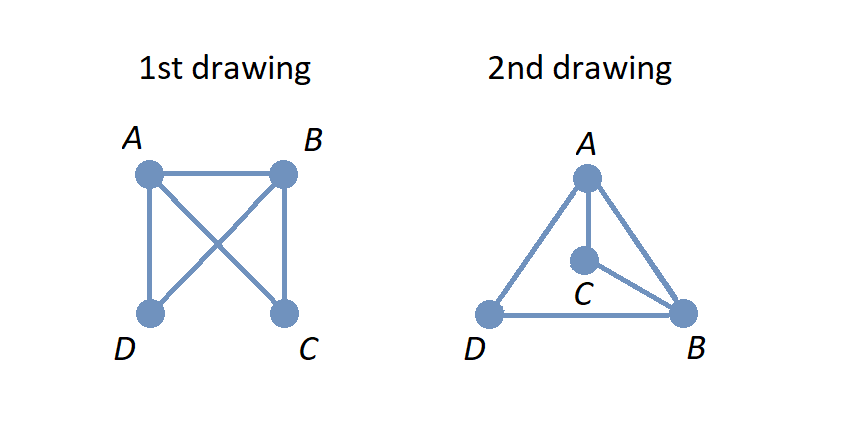
In the image, two different drawings are shown for the same graph. Notice that in each drawing, the connections between pairs of vertices are the same: The only pair of vertices that is not connected by an edge is \(\{ C, D \}.\)
Also notice that there is no vertex drawn where the two edges cross in the 1st drawing on the left, so this graph has 4 exactly vertices: \(A,\) \(B,\) \(C,\) and \(D.\)
A graph can represent relationships between pairs of people.
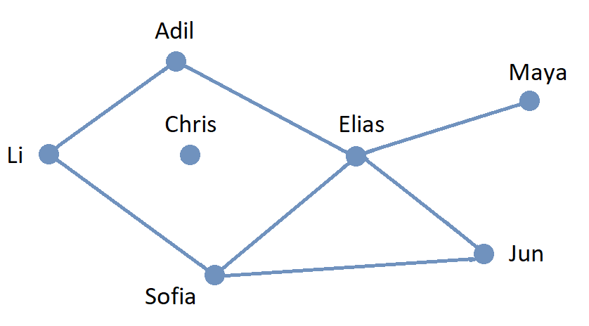
Here is a graph that represents whether pairs of students are enrolled in at least one class together. Each of the 7 vertices represents a student, and each of the 7 edges represents a pair of students who are enrolled in a class together.
The graph indicates that Adil and Elias are enrolled in at least one class together and that Elias and Maya are enrolled in at least one class together.
Here are some other examples of graphs.
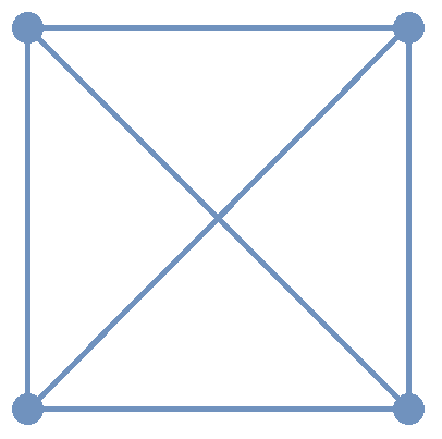
A complete graph is a graph in which every pair of distinct vertices are the endpoints of exactly one edge. The image shows the complete graph on 4 vertices. Notice that two edges appear to "intersect" but there is no vertex drawn where the edges cross, so these edges do not have any points in common - as stated above, an edge contains only its endpoints.
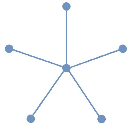
A star graph is a graph that has one central vertex that is one of the endpoints of every edge in the graph. The image shows the star graph on 6 vertices. The star graph is one example of a tree, a graph in which for every pair of distinct vertices there is exactly one path of edges that can be used to connect the vertices. Some of the many applications of trees in computer science will be discussed in the Trees chapter.
The design of this book is to introduce each concept informally, as was done for the preceding foundational ideas, then notice properties and patterns, generalize from what has been noticed, and formalize the ideas to prepare for even deeper analysis.
And congratulations if you read through all of those foundational mathematical ideas in this subsection and worked through all the Questions and Challenges! If you compare the list of ideas to the Table of Contents, you will see that you have touched on every one of the topics that will be discussed in this textbook!
1.2.3. On-Demand Math Resources and Library Of Functions Appendices
Two appendices to this textbook contain additional mathematics that you may need to review as you work your way through the textbook.
1.2.4. Do I Need To Know How To Program In Python?
You are NOT expected to know the Python programming language before you start this course.
As you’ve seen above, this textbook contains Python code snippets that are designed to aid your understanding of the mathematical concepts. It is NOT one of the goals of this textbook to teach you Python, but instead "just enough Python" to be able to examine, run, and alter the existing code snippets.
The appendices "An Introduction to Python" and "Python Syntax Examples" cover most of the basic concepts you will need from the Python programming language.
1.3. Applications of Discrete Mathematics
Remixer’s Note: This section is taken from the original “Discrete Math” book, with only a few minor edits.
Discrete mathematics is applied in many areas including the physical, engineering, and increasingly, the social sciences.
1.3.1. Applications to Applied Mathematics
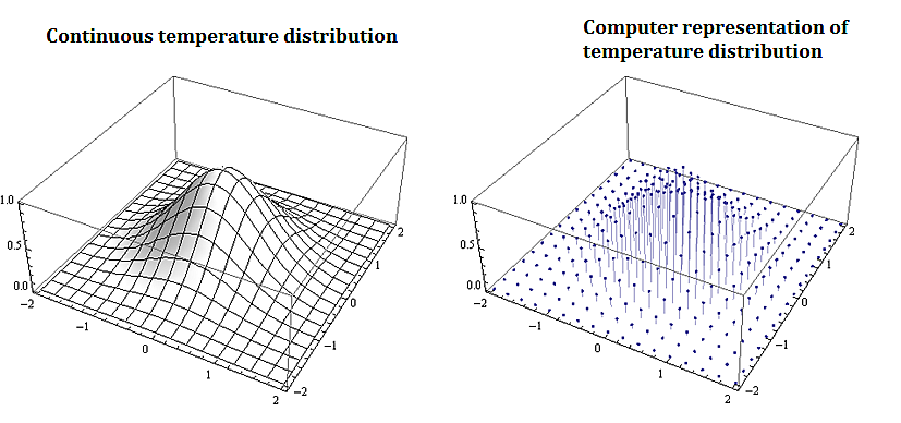
Most problems that involve computational methods, need to be solved using computers. Rather than solve for the temperature map of an entire planar region, we solve for the temperature using a discrete set of mesh or grid of points on a representative subset of the planar region.
1.3.2. Applications to Information Technology and Computer Science
Discrete mathematics is needed for computer science as information and data is stored digitally. Digitally represented data is inherently discrete and is processed using discrete methods. For example a course grid discrete representation of the 2-d temperature distribution from the plate above could be:
\( \left(\begin{matrix}1&1&1\\2&4&8\\3&9&27\\4&16&64\\5&25&125\\\end{matrix}\right) \)
A voter registry may have voters in a database accessible from a list:
\( \left(\begin{matrix}John\ Smith\\Raheem\ Johnson\\.\\.\\.\\Sarah\ Muller\\\end{matrix}\right) \)
Which may need to be accessed and sorted, say geographically or alphabetically.
1.3.3. Applications to Data Science
Data science solutions to many problems use machine learning algorithms that are inherently discrete in nature. The information that needs processing is discrete, as are the basic problems in data science such as classification or clustering problems. In particular
-
Information consisting of data sets is represented using various data structures including graphical structures such as trees. Data science methods and algorithms involve procedures that manipulate these graphical structures to, for example, networks, classification trees, and decision trees.
-
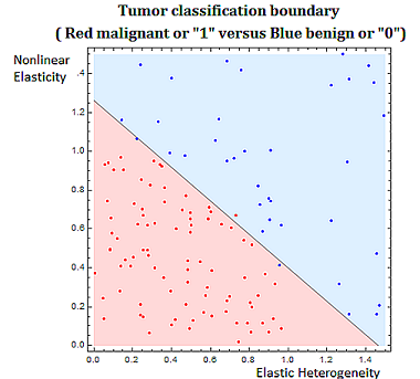
Classification problems are discrete in nature. Classifying tumors as malignant or as benign involves trying to predict if a variable \(Y\) that we can think of as taking on two values either \(0\) or \(1\) either malignant or benign. There are various algorithms used in classification problems, such as the binary tumor classification, including methods from probability.
1.3.4. Applications to Engineering
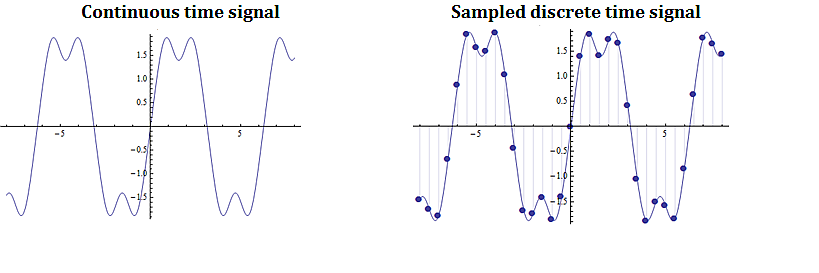
Digital signal processing involves taking a video, audio, or other signal like temperature, pressure, position and velocity, which is continuous, digitizing it and then processing the digital signal mathematically.
1.3.5. Applications of Combinatorics
Combinatorics involves in part the study of counting the number of objects, satisfying a specified condition, from sets of variable size. Enumeration and combinatorics is important in many areas and examples including:
-
Calculating the number of steps an algorithm needs to process a data set of variable size \(𝑛\). This problem is called the computational cost of the algorithm as a function of \(𝑛\).
-
Calculating the possible number of codes in a cryptographic code system
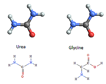
1.3.6. Applications of Graph Theory
Graph theory, which is the study of structures constructed with nodes and the edges joining them, has applications in many fields including,
-
Chemistry - representing molecular bonding and structure
-
Information technology and computer science - ranking pages on the internet, with pages considered as nodes and page links as edges.
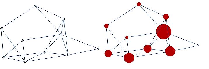
-
Industrial engineering and network optimization
-
Traffic routes (computer, internet, air, highway, subway systems) can be represented with stations as nodes and connections as edges.
-
Often we are interested in finding an optimal path in a network such as in the following example, finding the shortest tour over a series of towns on a map.
-
An example of the shortest tour problem, is shown below, using a software solution.

1.3.7. Applications of Probability and Statistics
Many probability assignments are based on counting and combinatorial methods.
-
If we assume that the likelihood of rain is the same on any day in the month of September, we might be interested in the probability that it rains on \(0\) days, it rains on exactly \(1\) day, exactly \(2\) days, etc. Such probability assignments are called discrete distributions, by contrast with continuous distributions like the bell curve.
-
Also probability and statistical techniques are often used in data science. The binary classification problem, of say classifying a tumor as malignant or benign, uses a statistical modeling technique, called regression, specifically logistic regression to determine the strength of the relationship between the independent variable, and dependent heterogeneity variable. In the tumor grading example the independent variable would be \((x_1,x_2 )\) (elastic heterogeneity, nonlinear elasticity), and the dependent variable would be \(Y\), classified as \(0\), or \(1\), (malignant or benign).
1.3.8. Applications to Social Sciences
Discrete mathematical techniques are important in understanding and analyzing social networks including social media networks.
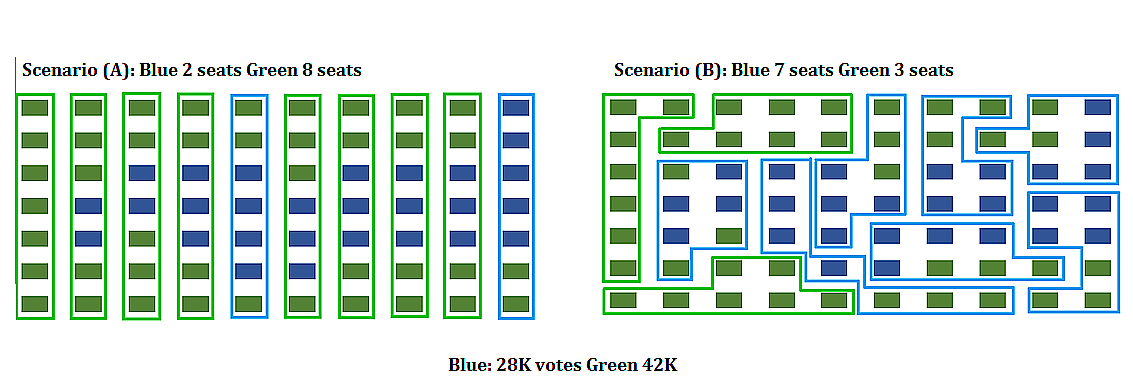
The mathematics of voting is a thriving area of study, including mathematically analyzing the gerrymandering of congressional districts to favor and/or disfavor competing political parties. The following example illustrates some of the fundamental ideas related to gerrymandering.
Consider a fictitious state made up of \(10\) congressional districts with \(7\) thousand voters in each district. To win a district a party (Green or Blue) needs to win \(4\) thousand or more votes. Consider the following two districting map scenarios. In each scenario, the blue party earns \(28\) thousand votes, and the green party earns \(42\) thousand votes. In scenario \(A\), the blue party wins \(2\) out of \(10\) districts, but in scenario \(B\) it wins \(7\) out of \(10\) districts.
1.4. Links to the Informal Definitions in this Chapter
For your reference in the future, here are direct links to most of the bullet points in the list of foundational ideas discussed in this section.
Sets, including subsets, the empty set, unions of sets, and intersections of sets
One-to-one correspondence, including the example "rock, paper, scissors"
Counting, including the Multiplication Principle and Pigeonhole Principle
Functions, including domain, codomain, range, inverse function, and the floor and ceiling functions \(\lfloor x \rfloor\) and \(\lceil x \rceil\)
Sequences, including index and terms
Recurrence Relations, including closed forms
Algorithms, including the Division Algorithm
2. Number Bases
NOTICE: If you are NOT enrolled in the CSC 230 course that I teach at SFSU, you probably are looking for the “public version” of the book, which I only update between semesters. The version you are looking at now is the “CSC230 version” of the book, which I will be updating throughout the semester.
This chapter was last updated on April 1, 2025.
It’s likely that you learned how to represent positive integers using the base-ten place-value system when you were young. This system uses ten symbols, the Hindu-Arabic numerals ‘0’, ‘1’, ‘2’, ‘3’, ‘4’, ‘5’, ‘6’, ‘7’, ‘8’, and ‘9’, to represent any natural number.
In the base-ten place-value system that uses decimal notation, each natural number is represented by a numeral which is a string of one or more of the ten Hindu-Arabic digits. However, in some computer science contexts, it is more useful to represent natural numbers in a place-value system that uses a different number base such as binary (base-two), octal (base-eight), or hexadecimal (base-sixteen). Using or thinking about numbers represented by numerals in these other systems can help you develop more efficient algorithms and recognize when certain numerals can be interpreted as encodings of multiple pieces of information.
In this chapter, you will learn how to represent natural numbers using place-value systems with bases other than ten.
Key terms and concepts covered in this chapter:
-
Number bases
-
binary
-
hexadecimal
-
octal
-
decimal
-
2.1. Numbers, Numerals, and Digits
In everyday life, it is common to treat numbers and numerals as if they are the same. However, it is important in this chapter to distinguish these concepts.
-
A number is an abstract idea or mental concept of a count, a measure, a rank in an ordering, etc..
-
A numeral is a word, phrase, symbol, or string of symbols that is used to represent a number.
-
A digit is a single symbol that represents a number. A digit is a numeral, but multiple digits can be combined to create other numerals. For example, each of the ten Hindu-Arabic numerals is a digit that represents a natural number that is less than ten, and multiple Hindu-Arabic numerals can be combined to create numerals that represent numbers that are greater than or equal to ten.
NOTE: The word "digit" comes from the Latin word digitus which means "finger" or "toe."
2.2. Review Of The Base-Ten Place Value System
It’s likely that everything you are about to read in this section is knowledge you’ve had for many years. The purpose of stating everything so explicitly is to provide an example you can compare with place-value systems that use other bases.
A base-ten numeral is a string formed from one or more digits (i.e., Hindu-Arabic numerals.)
-
The string is read from left-to-right.
-
Each digit in the string represents a multiple of a power of the base, ten, depending on the its position in the string.
-
The rightmost place represents a multiple of 1 (which is ten raised to the power zero) and each of the other places represents a multiple of a power of ten that is one greater than the power of ten represented by the place to its right.
-
Notice that the base itself, the number ten, is represented by the string "10" in this place-value system. The string "10" represents the number described by the phrase "1 ten plus 0 ones".
-
As an example, the string "101" represents the number described by the phrase "1 hundred plus 0 tens, plus 1 ones," where 1 hundred is the same as ten tens. That is, \[ 101 = 1 \cdot 10 \cdot 10 + 0 \cdot 10 + 1 \cdot 1 \] The expression on the right-hand side of the previous equation is referred to as expanded form in school-level mathematics.
NOTE: The Hindu-Arabic numerals evolved from earlier Brahmi versions. You can look at the image at this web page which shows a few steps in this evolution. Also, you can learn more about the history of the Hindu-Arabic numerals from the links in the "Notes" and "References" sections of this Wikipedia page.
2.2.1. An Algorithm That Computes The Digits Of A Base-Ten Numeral
In this subsection, an algorithm is presented for computing the digits in the expanded form of a base-ten numeral of the natural number \(n.\) This may seem to be a complicated way to do something very simple since we could just read off the digits, but the important thing to notice about this algorithm is that the role that ten plays can be played by any other positive integer constant greater than one! This means that this algorithm can be adapted to find the "digits" in the expanded form of a base-\(b\) numeral for the number \(n\) for any base \(b\) we choose.
-
Task: Given the natural number n, compute an array of natural numbers \(s = [ r_{0}, \, r_{1}, \, \ldots \, r_{k} \)] so that each of \(r_{0}, r_{1}, \ldots , r_{k}\) is represented by a single digit in base-10, and \[ n = r_{k} \cdot 10^{k} + \ldots + r_{1} \cdot 10^{1} + r_{0} \cdot 10^{0} \] where \(k\) is the greatest natural number such that \(10^{k} < n.\)
-
Input: The natural number \(n\)
-
Steps:
-
Set \(a\) equal to \(n\)
-
Set \(s\) to the empty array (We will append the values \(r_{0}, r_{1}, \ldots , r_{k}\) to the array \(s\) as we compute them)
-
Divide \(a\) by 10 to find natural numbers \(q\) and \(r\) such that both \(a = q \cdot 10 + r\) and \(0 \leq r < 10.\)
-
Append \(r\) to the end of array \(s.\)
-
If \(q \neq 0\)
-
set \(a\) equal to \(q\)
-
go to step 3
-
-
Return the sequence \(s.\)
-
-
Output: An array of natural numbers \(s = [ r_{0}, \, r_{1}, \, \ldots \, r_{k} \)] where each number is represented by a single digit, and \[ n = r_{k} \cdot 10^{k} + \ldots + r_{1} \cdot 10^{1} + r_{0} \cdot 10^{0}.\]
-
That is, we rewrite \(n\) as \(r_{0} + 10 \cdot (r_{1} + 10 \cdot (r_{2} + \ldots r_{k-1} + (10 \cdot (r_{k})) \ldots ))\)
2.3. The Base-Two Place Value System (Binary Notation)
This subsection describes the base-two (binary) place value system. You will see that much of what is written here is the result of replacing "ten" by "two" in the description of the base-ten (decimal) system in the previous section.
A base-two numeral is a string formed from one or more of the two binary digits (or bits) ‘0’ and ‘1’.
-
The string is read from left-to-right.
-
Each digit in the string represents a multiple of a power of the base, two, depending on the its position in the string.
-
The rightmost place represents a multiple of 1 (which is two raised to the power zero) and each of the other places represents a multiple of a power of two that is one greater than the power of two represented by the place to its right.
-
Notice that the base itself, the number two, is represented by the string "10" in this place-value system. The string "10" represents the number described by the phrase "1 two plus 0 ones".
-
As an example, the string "101" represents the number described by the phrase "1 four plus 0 twos, plus 1 ones," where 1 four is the same as two twos. That is, \[ 101 = 1 \cdot 10 \cdot 10 + 0 \cdot 10 + 1 \cdot 1 \text{ (🤯: Wait… WHAT?!?) }\] Yes, this equation, which may appear to be written in the base-ten system, is correct in the base-two place value system, too! "10" is how the number two is represented in base-two notation!
As an analogy, the string "pie" signifies different things in English (a baked dessert) and Spanish (a foot.) You must take care to know which context you are working in!
|
It is traditional to use some extra notation to indicate when the strings "10" and "101" are not base-ten numerals to avoid confusion. In this textbook, numerals in any base other than ten will be written between a pair of parentheses followed by a subscript indicating the base. The subscript is written as a base-ten numeral. For example, we could rewrite the previous equation as \[(101)_{2} = (1)_2 \cdot (10)_2 \cdot (10)_2 + (0)_2 \cdot (10)_2 + (1)_2 \cdot (1)_2 \] which translates into base-ten as \(5 = 1 \cdot 2 \cdot 2 + 0 \cdot 2 + 1 \cdot 1.\) We can also write \(5 = (101)_2\) which is a way of saying that the base-ten numeral and the base-two numeral signify the same number. + NOTE: The reason we use base-ten numerals as the subscripts on numerals in other bases is because base-ten is so dominant: It is the "privileged" base, so we need to indicate when a different base is being used… and we don’t need to use the parentheses or subscripts if we are already working in base-ten. |
|
The parentheses and subscript are not necessary if it is clear from the context that a numeral is not a base-ten numeral. For example, \[ \text{chmod 755 hello.txt} \]
is a Unix/Linux command that changes the file permission bits (read, write, execute) of the file "hello.txt" for the file’s owner, the file’s group, and any other user. In this example, the string "755" is not a base-10 numeral, but is in octal (base-eight). Octal will be discussed later in the chapter. No subscript is used in the Unix/Linux command because it is natural to an experienced user of that operating system to use octal in the context. Also, we can omit the parentheses and subscripts if we want to tell a couple of "jokes:" |
You are ready now to learn how to represent numbers using base-two numerals.
2.3.1. An Algorithm That Computes The Digits Of A Base-Two Numeral
In this subsection, an algorithm is presented for computing the digits in the expanded form of a base-two numeral of the natural number \(n.\) This algorithm has been adapted from the one stated for base-ten in the previous section. Notice that all numerals used in this algorithm are base-ten numerals unless otherwise indicated.
-
Task: Given the natural number n, compute an array of natural numbers \(s = [ r_{0}, \, r_{1}, \, \ldots \, r_{k} \)] so that each of \(r_{0}, r_{1}, \ldots , r_{k}\) is represented by a single digit in base-2, and \[ n = r_{k} \cdot 2^{k} + \ldots + r_{1} \cdot 2^{1} + r_{0} \cdot 2^{0} \] where \(k\) is the greatest natural number such that \(2^{k} < n.\)
-
Input: The natural number \(n\)
-
Steps:
-
Set \(a\) equal to \(n\)
-
Set \(s\) to the empty array (We will append the values \(r_{0}, r_{1}, \ldots , r_{k}\) to the array \(s\) as we compute them)
-
Divide \(a\) by 2 to find natural numbers \(q\) and \(r\) such that both \(a = q \cdot 2 + r\) and \(0 \leq r < 2.\)
-
Append \(r\) to the end of array \(s.\)
-
If \(q \neq 0\)
-
set \(a\) equal to \(q\)
-
go to step 3
-
-
Return the sequence \(s.\)
-
-
Output: An array of natural numbers \(s = [ r_{0}, \, r_{1}, \, \ldots \, r_{k} \)] where each number is represented by a single digit, and \[ n = r_{k} \cdot 2^{k} + \ldots + r_{1} \cdot 2^{1} + r_{0} \cdot 2^{0}.\]
-
That is, the algorithm rewrites \(n\) as \(r_{0} + 2 \cdot (r_{1} + 2 \cdot (r_{2} + \ldots r_{k-1} + (2 \cdot (r_{k})) \ldots ))\)
Here is a link to an alternate method of finding the base-two numeral for a number.
If you made it to this sentence without skipping any of the discussion above, congratulations! If you did skip some of the discussion, go back and try your best to understand what the algorithm in the previous example is computing: The array \(s\) holds the digits, in reverse order of the binary notation for the number \(n.\) Compare what is done in this algorithm to the one for base-ten in the previous section… they are computing the digits for a numeral, but in different bases. If you can understand this algorithm, you will likely understand the rest of the chapter.
2.4. The Base-\(b\) Place Value System
If you made it here, you are ready to learn how to find, given any natural number \(n,\) the numeral that represents \(n\) in the base-\(b\) place value system (It is assumed that the base \(b\) is a natural number greater than or equal to 2.) You can compare the algorithm and example in this subsection to the ones in the preceding subsections for base-ten and base-two.
A base-\(b\) numeral is a string formed from one or more digits out of a set that contains \(b\) symbols, where each symbol is called a "base-\(b\) digit."
-
The string is read from left-to-right.
-
Each digit in the string represents a multiple of a power of the base, \(b,\) depending on the its position in the string.
-
The rightmost place represents a multiple of 1 (which is \(b\) raised to the power zero) and each of the other places represents a multiple of a power of \(b\) that is one greater than the power of \(b\) represented by the place to its right.
-
Notice that the base itself, the number \(b,\) is represented by the string "10" in the base-\(b\) place value system. The string "10" represents the number described by the phrase "1 \(b\) plus 0 ones".
-
As an example, the string "101" represents the number described by the phrase "1 b-_squared plus 0 _b, plus 1 ones." That is, \[ 101 = 1 \cdot 10 \cdot 10 + 0 \cdot 10 + 1 \cdot 1 \text{ (🤯: Again?!?) }\] Yes, this equation is correct, too, in the base-b place value system!
To avoid confusion, you can enclose each numeral in a pair of parentheses followed by the subscript \(b\) to indicate the base, where \(b\) is written as a base-ten numeral. For example, the previous equation can be written as \[(101)_{b} = (1)_b \cdot (10)_b \cdot (10)_b + (0)_b \cdot (10)_b + (1)_b \cdot (1)_b \] which translates into base-ten as \(b^2 + 1 = 1 \cdot b \cdot b + 0 \cdot b + 1 \cdot 1.\)
2.4.1. An Algorithm That Computes The Digits Of A Base-\(b\) Numeral
This is an adaptation of the algorithm presented earlier for base-two. Notice that all numerals used in this algorithm are base-ten numerals unless otherwise indicated.
-
Task: Given the natural number n, and positive integer constant \(b > 1\) compute an array of natural numbers \(s = [ r_{0}, \, r_{1}, \, \ldots \, r_{k} \)] so that each of \(r_{0}, r_{1}, \ldots , r_{k}\) can be represented by a single digit in base-\(b\), and \[ n = r_{k} \cdot b^{k} + \ldots + r_{1} \cdot b^{1} + r_{0} \cdot b^{0} \] where \(k\) is the greatest natural number such that \(b^{k} < n.\)
-
Input: The natural number \(n\)
-
Steps:
-
Set \(a\) equal to \(n\)
-
Set \(s\) to the empty array (We will append the values \(r_{0}, r_{1}, \ldots , r_{k}\) to the array \(s\) as we compute them)
-
Divide \(a\) by \(b\) to find natural numbers \(q\) and \(r\) such that both \(a = q \cdot b + r\) and \(0 \leq r < b.\)
-
Append \(r\) to the end of array \(s.\)
-
If \(q \neq 0\)
-
set \(a\) equal to \(q\)
-
go to step 3
-
-
Return the sequence \(s.\)
-
-
Output: An array of natural numbers \(s = [ r_{0}, \, r_{1}, \, \ldots \, r_{k} \)] where each number is represented by a single digit in base-\(b,\) and \[ n = r_{k} \cdot b^{k} + \ldots + r_{1} \cdot b^{1} + r_{0} \cdot b^{0}.\]
-
The algorithm rewrites \(n\) as \(r_{0} + b \cdot (r_{1} + b \cdot (r_{2} + \ldots r_{k-1} + (b \cdot (r_{k})) \ldots )).\) The result \(s\) contains the numbers that let you write \(n\) in base-\(b\) notation.
2.4.2. Octal Notation (Base-8)
2.4.3. Hexadecimal Notation (Base-16)
2.4.4. A Theorem (To Be Proven Later)
We can summarize what the algorithm does as a mathematical theorem, though technically at this point, it’s only a conjecture, an educated guess based on a few cases that seem to indicate that the algorithm will always work. You will learn a technique that will prove the theorem by validating the algorithm for all choices of natural numbers \(n\) and \(b>1\) in the Proofs: Mathematical Induction chapter.
2.5. Converting From Base-\(b\) to Base-Ten
In this section you will learn how to rewrite a base-\(b\) numeral in base-ten.
Several common bases used in computer science are base \(2\), base \(8\), and base \(16\), which are referred to as binary, octal, and hexadecimal, respectively. Binary digits are often referred to as bits. Note that, when finding the hexadecimal expansion of a positive integer, in addition to the usual digits \(0\) through \(9,\) we require an additional 6 digits. We will represent these by the letters \(\mathrm{A}\) through \(\mathrm{F}\), where \((\mathrm{A})_{16} = 10,\) \((\mathrm{B})_{16} = 11,\) \((\mathrm{C})_{16} = 12,\) \((\mathrm{D})_{16} = 13,\) \((\mathrm{E})_{16} = 14,\) and \((\mathrm{F})_{16} = 15.\)
2.6. Base Conversion Among Binary, Octal, and Hexadecimal
One of the ways that octal (base-eight) and hexadecimal (base-sixteen) are used in computer science is to abbreviate long bitstrings. The following examples will show how this is done.
Suppose you need to convert a numeral from hexadecimal to binary. One method would be to first convert from hexadecimal to decimal, and then convert the result from decimal to binary. However, it is much more efficient to notice that since \(2^4 = 16,\) you can express each hexadecimal digit as a block of 4 bits (that is, a bitstring of length 4) as follows:
You can then concatenate the blocks, and remove any leading zeros if you need to.
To convert a numeral from binary to hexadecimal, first break up the binary notation into blocks of 4 bits, adding a suitable number of leading zeros if necessary. Next, convert each block of 4 bits to a hexadecimal digit and concatenate the results, removing any leading zeros if necessary.
A similar method can be used to convert between octal and binary. Since \(2^3 = 8,\) each octal digit can be written uniquely as a block of 3 bits as follows:
We then concatenate blocks, removing any leading zeros if necessary.
Also, the following table can be used to covert quickly between decimal, hexadecimal, octal, and binary in a similar way.
Conversion table for different bases
Decimal |
0 |
1 |
2 |
3 |
4 |
5 |
6 |
7 |
8 |
9 |
10 |
11 |
12 |
13 |
14 |
15 |
Hexadecimal |
0 |
1 |
2 |
3 |
4 |
5 |
6 |
7 |
8 |
9 |
A |
B |
C |
D |
E |
F |
Octal |
0 |
1 |
2 |
3 |
4 |
5 |
6 |
7 |
10 |
11 |
12 |
13 |
14 |
15 |
16 |
17 |
Binary |
0 |
1 |
10 |
11 |
100 |
101 |
110 |
111 |
1000 |
1001 |
1010 |
1011 |
1100 |
1101 |
1110 |
1111 |
2.7. Exercises
-
Convert to decimal (base 10)
-
\((10262)_7\)
-
\((30A8)_{16}\)
-
\((1000010001100)_2\)
-
\(({12307)}_{60}\)
-
-
Convert \(\left(2039\right)_{10}\) from decimal (base 10) to
-
base 7
-
binary
-
hexadecimal (base 16)
-
octal (base 8)
-
-
Convert \(\left(2599\right)_{10}\) from decimal to
-
base 5
-
binary
-
hexadecimal
-
base 3
-
-
Convert the following hexadecimal numerals to binary numerals
-
\(\left(6F203\right)_{16}\)
-
\(\left(3FA20C45\right)_{16}\)
-
\(\left(FACE\right)_{16}\)
-
-
Convert the following binary numerals to hexadecimal numerals
-
\(\left(1111100111010101101\right)_2\)
-
\(\left(\ 10001111101011\right)_2\)
-
\(\left(1100101011111110\right)_2\)
-
3. Counting: Arithmetic Techniques
NOTICE: If you are NOT enrolled in the CSC 230 course that I teach at SFSU, you probably are looking for the “public version” of the book, which I only update between semesters. The version you are looking at now is the “CSC230 version” of the book, which I will be updating throughout the semester.
This chapter was last updated on February 2, 2025.
Contents locked until 11:59 p.m. Pacific Standard Time on May 23, 2025.
You probably learned how to count objects one by one when you were a child. You may have counted up to 5 on the fingers on one hand, or up to 10 on the fingers of two hands, or up to 20 on fingers and toes - that is, you paired the objects (fingers and/or toes) with number names to create a one-to-one correspondence. You may have counted all the way up to 100.
However, many problems in computer science or mathematics require you to count the number of elements in sets that contain millions of elements, or billions of elements, or even more elements, so counting one by one is inefficient or impossible. Starting with this chapter, and continuing later in the Set Theory and Counting: Permutations and Combinations chapters, you will study ways to quickly and efficiently count the number of elements of any set no matter the size of the set.
Key terms and concepts covered in this chapter:
-
Counting arguments
-
Sum Rule
-
Product Rule
-
Division Rule (also called the Rule Of Quotient)
-
Subtraction Rule (also called the Principle of Inclusion-Exclusion for two sets)
-
-
The pigeonhole principle
3.1. Some Foundational Counting Principles
Each of the four arithmetic operations corresponds to a rule we can use to count quickly.
3.1.1. The Sum Rule
The sum rule, also called the addition principle or the rule of sum, describes the number of possible choices of one element from a union of two sets that share no common elements (Such sets are called disjoint sets).
This is called the sum rule for counting because it involves adding to find a total. The sum rule can also be extended to more than two sets, as long as every pair of the sets have no elements in common.
A student in a Capstone course can choose a project from three different professors. The professors have 3, 7, and 4 possible projects, and no project is on more than one professor’s list. How many possible projects can the student choose?
The student can pick out a project by choosing from the first professor, the second professor, or the third professor. Since no project is on more than one list, the sum rules says that there are \(3 + 7 + 4 = 14\) projects to choose from.
A card
will be
drawn from a standard 52-card deck.
How many ways can the card be an even number or a king?
Image credit: This is a cropped version of "Set Of Playing Card". George Hodan has released this “Set Of Playing Card” image under Public Domain license (CC0 Public Domain).
3.1.2. The Subtraction Rule
The subtraction rule describes the number of possible choices of one element from a union of two sets that do share one or more common elements.
The subtraction rule is a special case of the inclusion-exclusion principle that involves only two sets. The inclusion-exclusion principle is discussed in more detail in the Set Theory and Proofs: Mathematical Induction chapters.
Video Example
The following video example features Dr. Joshua Roberts, Associate Professor of Mathematics at Georgia Gwinnett College.
Notice that Dr. Roberts uses a Venn diagram to represent the sets in this video. Venn diagrams are covered in the Set Theory chapter of the Remix.
3.1.3. The Product Rule
The product rule, also called the multiplication principle or the rule of product, describes the number of possible choices of two successive elements where the first element comes from one set and the second from another set (which could be the same set as the first set).
To find the total number of outcomes for two or more successive events where both events must occur, multiply the number of outcomes for each event together. For instance, if you want to find the number of outcomes possible when you roll a die and toss a coin, you could use the product rule. It is important to note that the events must be independent, meaning one doesn’t effect the other.
Video Example
The following video example features Dr. Joshua Roberts, Associate Professor of Mathematics at Georgia Gwinnett College.
3.1.4. The Division Rule
This rule is used when there are \(n\) ways to complete a procedure, but each of those ways is equivalent to \(d\) ways (including the way itself.) That is, every possible outcome of the procedure can be done in \(d\) different ways
The next example uses both the product and division rules.
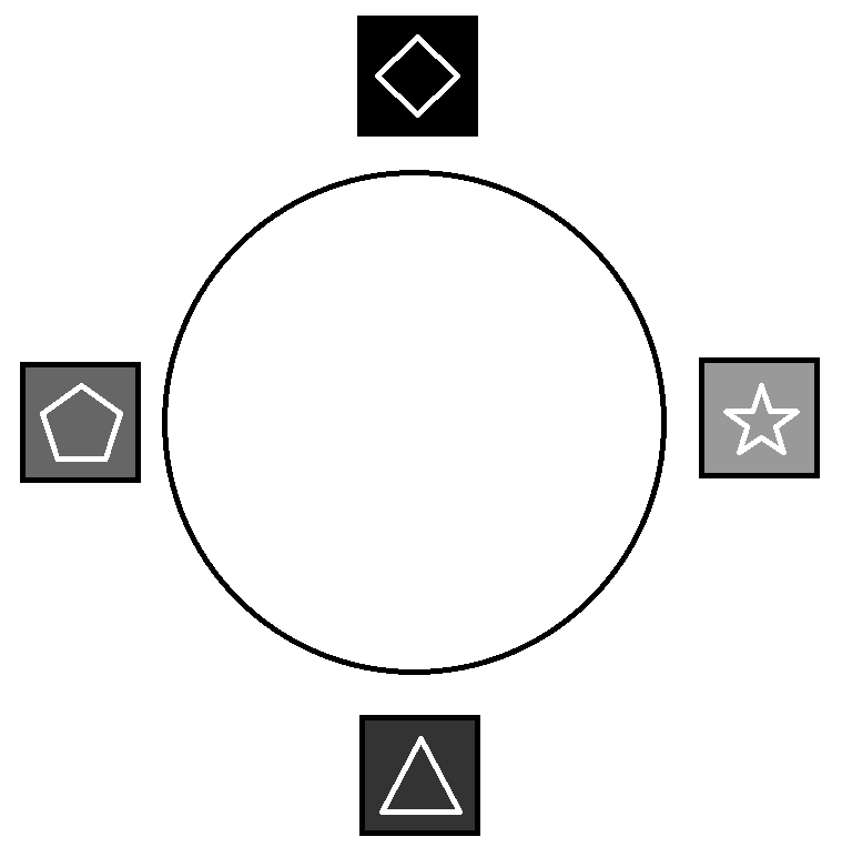
Four students will sit around a circular table, but two seatings are considered "not different" whenever each student has the same left neighbor and right neighbor. How many different seatings are there?
First use the product rule to find that there are (4)(3)(2)(1) = 24 possible ways for the 4 students to sit (For example, there are 4 choices for the "North," then 3 choices remaining for the "East," then 2 choices remaining for the "South," and 1 choice remaining for the "West.") Next, notice that if all the students shifted one chair to the left once, twice, or thrice, they would all have the same neighbors that they originally had. This means that for each of the 24 ways the students can sit, 4 of those ways are not considered different.
Therefore, there are \(\frac{24}{4}\) or 6 different seatings.
3.2. The Pigeonhole Principle
A suprising number of counting problems can be solved with the so-called pigeonhole principle.
Click here to see a photoshopped image that illustrates this principle.
3.3. Exercises
-
There are 67 mathematics majors and 124 computer science majors at a college. There is no student who is both a mathematics major and a computer science major.
-
In how many ways can two representatives be picked so that one is a mathematics major and one is a computer science major?
-
In how many ways can one representative be picked who is either a mathematics major or a computer science major?
-
-
A multiple-choice test contains 20 questions, and each question has four choices.
-
In how many ways can a student answer all of the questions on the test if each question must be answered?
-
In how many ways can a student answer all of the questions if the student is allowed to not answer one or more questions?
-
-
How many different three-letter initials, using uppercase English letters, are there?
-
How many different three-letter initials, using uppercase English letters, end with "R"?
-
How many bit strings are there of length five?
-
How many bit strings are there of length five that begin and end with 1?
-
How many bit strings are there of length less than \(n\), where \(n\) is a positive integer, that start and end with 1?
-
How many license plates can be made using three digits followed by four uppercase English letters if:
-
Digits and letters can be repeated?
-
Digits and letters cannot be repeated?
-
-
Each student in a Discrete Mathematics class is a mathematics major, a computer science major, or a double major in both mathematics and computer science. If the class has 5 mathematics majors (including double majors), 23 computer science majors (including double majors), and 7 double majors, how many students are in the class?
-
Suppose a computer system requires a password of length no less than 7 and no more than 10 characters, and each character must be an English lowercase letter, an English uppercase letter, a digit, or one of six special characters (*, >, <, !, +, =).
-
How many different passwords are available?
-
Suppose a hacker can check a potential password once every nanosecond (1 nanosecond is \(1 \times 10^{-9}\) seconds). How long will it take the hacker to check every potential password?
-
-
Suppose that there are 29 students in a class, all of whose last names use only English letters. Explain why at least 2 students in the class have last names that begin with the same letter.
-
Show that in any set of 5 integers, there are at least two of them that have the same remainder when divided by 4.
-
A bag contains 8 red balls and 7 blue balls.
-
How many balls must be chosen to be sure of choosing 3 of the same color?
-
How many must be chosen to be sure of choosing 3 red balls?
-
-
Someone cleaning out their attic finds a box containing 12 rock CDs and 12 country CDs. What is the minimum number of CDs they can take out to guarantee at least one of each type?
-
Give an argument that there are at least two people in California with the same number of hairs on their head.
4. Set Theory
NOTICE: If you are NOT enrolled in the CSC 230 course that I teach at SFSU, you probably are looking for the “public version” of the book, which I only update between semesters. The version you are looking at now is the “CSC230 version” of the book, which I will be updating throughout the semester.
This chapter was last updated on September 15, 2025.
Fixed some typos.
Set theory, along with logic, is the foundation of mathematics in our time. In earlier eras, people tried to use arithmetic (e.g., counting and whole numbers) and geometry (e.g., measurement of lengths, areas, and volumes along with geometric constructions) as the foundations of all mathematics. However, over the last two centuries, mathematicians gained new understandings of issues with these traditional foundations which led them to seek a new, firmer foundation. For now, that firmer foundation uses set theory: The study of collections of objects and how those collections can be combined, associated, and themselves added to other collections.
NOTE: If you want to dig much more deeply into what the issues with using arithmetic or geometry as the foundation of mathematics are, you can start with this Wikipedia page which includes a a brief description of the "foundational crisis of mathematics."
Key terms and concepts covered in this chapter:
-
Sets
-
Subsets of a set
-
The empty set
-
The power set of a set
-
Cartesian products
-
-
Venn diagrams
-
Cardinality and countability of finite and infinite sets
-
Set cardinality and counting
-
-
Operations with sets: Union, intersection, complement, and others
-
DeMorgan’s laws
-
Inclusion-exclusion principle
-
4.1. Sets
A set is an unordered collection of objects, called elements or members. A set is said to contain its elements.
If \(x\) is an element of the set \(S,\) then we write \(x \in S\). If \(x\) is not an element of the set \(S\), then we write \(x \not\in S\). For example, if \(S\) is the set of names of states in the United States of America, then “New York” is an element of \(S\) and “Ontario” is not an element of \(S,\) that is \[ \text{“New York”} \in S \text{ and } \text{“Ontario”} \not\in S. \] As another example, if \(E\) is the set of even integers, then \(2 \in E\) and \(3 \not\in E.\)
4.1.1. Describing A Set: The Roster Method
One way of describing a set is the roster method: List all the elements of the set between curly braces. For example, \[A = \{1,-2,0,1,-3\} \] is the set whose elements are \(-3,\) \(-2,\) \(0,\) and \(1.\)
-
Notice that the set \(A\) contains exactly \(4\) elements, even though the element \(1\) appears twice in the roster - duplicate entries do not matter.
-
Also, the order of the elements in the list does not matter. That is, \(\{-3,-2,0,1 \}\) and \(\{0, 1,-2,-3\}\) are two more ways of describing the same set \(A.\)
|
A WARNING ABOUT THE PYTHON EXAMPLES INVOLVING SETS: The mathematical set \(A = \{1,-2,0,1,-3\}\) is a constant - you cannot change the set by removing elements or inserting new elements. However, Python objects of type set are mutable so it is possible to remove elements or insert new elements, as shown in the following code example. The mathematically correct implementation of sets in Python uses objects of type frozenset because objects of type frozenset are immutable, just like mathematical sets. But there are advantages to using type set instead of frozenset: The roster method notation can be used to initialize or print a Python set, but cannot be used with a Python frozenset: You must call the frozenset constructor to create and initialize a frozenset. The authors of the original “Discrete Math” chose to use Python sets instead of frozensets in the code examples; the author of this remix made the same choice. |
4.1.2. Describing A Set: Set Builder Notation
Another way of describing a set is the use of set builder notation. We write a set as \[\{x \in D : P(x)\}.\] This is the set of all elements \(x\) from a domain \(D\) that satisfy the predicate \(P(x).\) We can use either the colon \(:\) or the vertical bar \(|\) as the separator in this notation. For example, \(\{ x \in \mathbb{N} \, | \, x^{2} \leq 50 \}\) is the set of natural numbers that are less than \(\sqrt{50}.\)
Yet another way of describing a set is to use a function or an algebraic expression, as in \[\{ f(x) : x \in D \}.\]This is the set of all values \(f(x)\) for \(x\) in the domain \(D\). For example, \(\{ 2n : n \in \mathbb{N} \}\) is the set of the even natural numbers. Again, we can use either the colon \(:\) or the vertical bar \(|\) as the separator.
4.1.3. Describing A Set: Special Sets Of Numbers
You may already be familiar with the following sets of numbers, which are listed here for reference.
Other special sets will be defined as needed.
4.1.4. Describing A Set: Switching Between Representations
A set can usually be described in more than one way, as shown in the following example.
|
When there are too many elements in a set for us to be able to list each one, we often use ellipses (\(\dots\)) when the pattern is obvious. For example, we have \[\mathbb{Z} = \{\dots,-3,-2,-1,0,1,2,3,\dots\}.\] |
4.2. Equality Of Sets
We say that two sets are equal if and only if they contain the same elements. When \(A\) and \(B\) are equal sets, we write \(A = B\). When \(A\) and \(B\) are not equal sets, we write \(A \neq B\).
The three sets \(\{2,3,5,7\},\) \(\{5,2,7,3\},\) and \(\{x \in \mathbb{N} : x \text{ is prime and } x < 10 \}\) are equal sets because they contain the same elements. In fact, \(\{2,3,5,7\},\) \(\{5,2,7,3\},\) and \(\{x \in \mathbb{N} : x \text{ is prime and } x < 10 \}\) are really just three different descriptions of the same set, in the same way that
\(1 + 3,\) \(5 - 1,\) and \(2^{2}\) are three different descriptions of the same number, 4.
The extended equality \[\{2,3,5,7\} = \{5,2,7,3\} = \{x \in \mathbb{N} : x \text{ is prime and } x < 10 \}\] is a true statement for the same reason the extended equality \(1 + 3 = 5 - 1 = 2^{2}\) is a true statement.
Note: You may be used to using the equal sign "=" as if it means "simplifies to" in your previous math experience, but "=" actually means "represents the same thing as."
4.3. The Empty Set
Consider the set of all natural numbers whose square is equal to 2, described using set builder notation: \(\{x \in \mathbb{N} : x^2 = 2\}.\) If you use the roster method to list all the elements you will get the set \(\{ \}\) because there are no natural numbers whose square is equal to 2!
The set \(\{ \}\) is called the empty set, or the null set. The symbol \(\emptyset\) is used to represent the empty set, too, that is, \[ \emptyset = \{ \}. \]
|
It is important to note that \(\{\}\) and \(\emptyset\) are both ways to write the empty set. However, the mathematical set \(\{ \emptyset \}\) is not the empty set because it contains one element, namely the empty set. In general, the set \(A\) is not the same as the set \(\{ A \}.\) |
|
Python Tip: The mathematical set \(\{ \emptyset \}\) must be implemented as \(\{ \text{frozenset()} \}\), which is the Python set that contains the empty frozenset. In general, anytime we want to implement a mathematical set \(B\) as an element of another mathematical set \(A\) in Python, we need to implement \(B\) as a frozenset in order to be used as an element of the Python set \(A\). This is due to the fact that elements of Python sets must be hashable; further explanation is beyond the scope of this textbook. |
4.4. Subsets of a Set
Suppose \(A\) and \(B\) are two sets, and that every element \(x\) of the set \(A\) is also an element of set \(B.\) We say that \(A\) is a subset of a set \(B,\) and write \(A \subseteq B\). If a set \(C\) is not a subset of \(B,\) we write \(C \not\subseteq B\).
If \(A \subseteq B\) but \(B\) contains at least one element that is not in A, then \(A\) is called a proper subset of \(B\), denoted \(A \subset B\). That is, \(A\) is a proper subset of \(B\) if it is a subset of \(B\) but is not equal to \(B.\)
4.5. The Power Set of a Set
Given a set \(A,\) we can define a new set by collecting together all subsets of \(A\). This new set is called the power set of \(A.\) The power set of \(A\) is denoted by \(\mathcal{P}(A).\) That is, \[ \mathcal{P}(A) = \{ B \, | \, B \subseteq A \}. \] Notice that \(\mathcal{P}(A)\) is a set whose elements are themselves sets.
The empty set has only one subset, namely itself. Thus, we see that \[\mathcal{P}(\emptyset) = \{\emptyset\}.\]
We can also find the power set of a power set. For example, we have the following:
| \[\begin{split} \mathcal{P}(\{ 3 \}) &= \{\emptyset, \{ 3 \}\},\\ \\ \mathcal{P}(\mathcal{P}(\{ 3 \}) &= \mathcal{P}(\{\emptyset, \{ 3 \})\\ &= \{\emptyset, \{\emptyset\}, \{ \{ 3 \} \}, \{\emptyset, \{ 3 \}\}\}. \end{split}\] |
4.6. Cartesian Products
The Cartesian product of two sets \(A\) and \(B\) is the set of ordered pairs defined by,
\( A\times B=\{(a,b) \, | \, a\in A \text{ and } b\in B)\}\),
|
Cartesian products are created using ordered pairs, so if \(A\) and \(B\) are different sets, then \(A \times B\) is different from \(B \times A\). |
|
The Cartesian coordinate systems are Cartesian products. The two-dimensional \(xy\)-plane is represented by \(\mathbb{R}^2=\mathbb{R}\times \mathbb{R}=\{(x,y)|x,y\in \mathbb{R}\}\), and, the three-dimensional \(xyz\)-space are represented by \(\mathbb{R}^3=\mathbb{R}\times \mathbb{R}\times \mathbb{R}=\{(x,y,z)|x,y,z\in \mathbb{R}\}\) |
4.7. Cardinality Of Sets: Finite Sets
Cardinality is the formalization of the idea of the count of the number of elements in a set.
In this section, we will prefer counting from 1 instead of 0. You will see below why this makes no difference.
Set \(A\) is called a finite set if either
-
\(A\) is the empty set or
-
there is a one-to-one correspondence between \(A\) and the set \(\{ i \in \mathbb{N} \, | \, 0 < i \leq n \} = \{1, 2, \ldots , n \}\) for some positive integer \(n.\)
|
This definition of "finite set" may seem abstract, but it’s just a formal description of what is likely the way you learned to count when you were young: You matched objects with number names (that is, numerals) as shown in the image. |
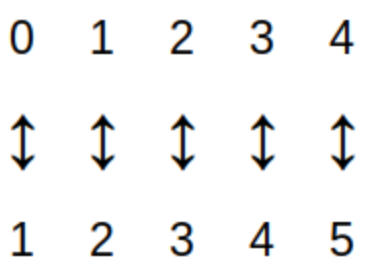
The cardinality of a finite set \(A,\) denoted by \(|A|,\) is
-
0 if \(A = \emptyset\) or
-
the value of \(n\) for which there is a one-to-one correspondence between \(A\) and \(\{1, 2, \ldots , n \}.\)
For a finite set \(A\) the cardinality \(|A|\) is just the number of elements in the set. The image shows that \(|\{0,1,2,3,4\}| = 5.\)
4.8. Venn Diagrams
A Venn diagram, named after the English mathematician John Venn, consists of one or more circles, with each circular region representing a set. An example can be seen here.
We write the elements of a set within the circular region that represents the set; anything written outside the circular region is not an element of the set. If an element is written in the overlap of two or more regions, then it is an element of each of the sets.
The circles are often drawn inside a larger rectangle which represents a universal set \(U\) that we are focusing on. In the example linked above, the rectangle was omitted because every glyph was an element of at least one of the sets represented by a circular region, but if we introduced addition glyphs like ہ we would need to draw the rectangle because that glyph would need to be written outside all three circular regions.
In this textbook, a Venn diagram must show all the possible overlaps of the sets. This is consistent with Venn’s paper from 1880.
That is, you should NOT be able to answer the question "Is x an element of set A?" when x is written in the circular region for a different set, B.
In the image, the upper right example shows a Venn diagram because you could write x in the overlap of the two regions or you could write x in the the part of the region for B that is outside the circular region for A. The lower two diagrams are not Venn diagrams: In either one of those, if x is written in the region for set B, it must be true that x is not an element of A (on the lower left) or that x is an element of A (the example on the lower right). Diagrams like the lower two examples will be called Euler diagrams in this textbook.
Some sources use the term Venn diagram for all four of the examples shown in the image, but you should always assume when reading this textbook that the lower two are NOT Venn diagrams. Click here to see the light!
4.9. Set Operations
We can obtain new sets by performing operations on other sets. When performing set operations, it is often helpful to consider all of our sets as subsets of a universal set \(U.\) We can think of the universal set as the set of all of the objects under consideration.
We can represent set operations visually using Venn diagrams.
4.9.1. Union
The union of the sets \(A\) and \(B\) is the set containing those elements that are in \(A\) or \(B\) or both, and is denoted by \(A \cup B\). More formally, \[A \cup B = \{x \in U : x \in A \text{ or } x \in B\}.\]
Note that "or" is read here as the "inclusive or". We have the following Venn Diagram for \(A \cup B\):
Note that, for any sets \(A\) and \(B,\) \[A \cup B = B \cup A.\]
4.9.2. Intersection
The intersection of the sets \(A\) and \(B\) is the set containing those elements that are in \(A\) and \(B\) and is denoted by \(A \cap B\). More formally, \[A \cap B = \{x \in U : x \in A \text{ and } x \in B\}.\]
We have the following Venn Diagram for \(A \cap B\):
Note that, for any sets \(A\) and \(B,\) \[A \cap B = B \cap A.\] If it is the case that \(A \cap B = \emptyset,\) then we say that \(A\) and \(B\) are disjoint. In other words, two sets are disjoint if and only if they contain no elements in common.
4.9.3. Complement
The complement of a set \(A\) is the set of all elements in the universal set \(U\) which are not elements of \(A\) and is denoted by \(\overline{A}.\) More formally, \[\overline{A} = \{x \in U: x \not\in A\}.\] Note that other textbooks and internet sources may use different notation for the complement of \(A\), such as \(A'\) and \(A^{c}\), but these all stand for the same set, so that \(\overline{A} = A' = A^{c}\).
We have the following Venn Diagram for \(\overline{A}\):
For any set \(A,\) \[ \overline{\overline{A}} = A \] \[ \overline{A} \cup A = U \] \[ \overline{A} \cap A = \emptyset. \]
4.9.4. Other Operations
The three operators complement, intersection, and union are the most commonly used to define subsets of a universal set. You will see why this is so later in the chapter.
However, there are some other operators you should be familiar with.
Difference
The difference of the sets \(A\) and \(B\) is the set containing those elements that are in \(A\) but not in \(B\) and is denoted by \(A \setminus B\). Set difference is also denoted by \(A - B\). More formally, \[A \setminus B = \{x \in U: x \in A \text{ and } x \not\in B\}.\]
We have the following Venn Diagram for \(A \setminus B\):
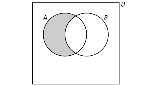
Note that, for any sets \(A\) and \(B\), if \(A \neq B,\) then \[A \setminus B \neq B \setminus A.\] However, if \(A = B,\) then \(A\setminus B = B \setminus A = \emptyset\).
Symmetric Difference
The symmetric difference of the sets \(A\) and \(B\) is the set containing those elements that are in \(A\) or \(B\) but not both \(A\) and \(B\). It is denoted by \(A \oplus B\) in this textbook, but other books and sources may use different notation such as \(A \Delta B\). More formally, \[A \oplus B = \{x \in U: (x \in A \text{ and } x \not\in B) \text{ or } (x \in B \text{ and } x \not\in A)\}.\]
We have the following Venn Diagram for \(A \oplus B\):
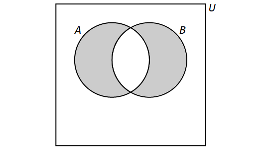
Note that, for any sets \(A\) and \(B,\) \[A \oplus B = B \oplus A.\]
4.9.5. Multiple Set Operations
We can also perform more than one set operation on a collection of sets. For example, let \(A,\) \(B,\) and \(C\) be sets and consider the following set: \[(A \setminus B) \cup (C \setminus B).\]This is the set that is obtained by taking the union of the sets \(A \setminus B\) and \(C \setminus B.\) We have \[(A \setminus B) \cup (C \setminus B) = \{x \in U: (x \in A \text{ and } x \not\in B) \text{ or } (x \in C \text{ and } x \not\in B)\}.\]
We have the following Venn Diagram for \((A \setminus B) \cup (C \setminus B)\):
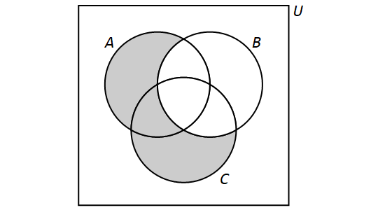
Note that the Venn Diagram also represents \((A \cup C ) \setminus B\). In general, there are multiple ways to describe the result of multiple set operations.
Video Examples
The following two video examples feature Dr. Katherine Pinzon, Professor of Mathematics at Georgia Gwinnett College.
Video Example 1
Video Example 2
4.10. Set Identities
Here is a collection of additional properties of the operations on sets. Each of these can be verified by drawing two Venn diagrams, one that represents the left-hand side of the equation and another that represents the right-hand side of the equation and showing that the resulting shadings of the Venn diagrams are the same.
Note that it is traditional to focus on complement, union, and intersection as the three primary set operations because the other operations such as difference and symmetric difference can be written in terms of those three primary operations, for example, \(A \setminus B = A \cap \overline{B}\) and \(A \oplus B = (A \cap \overline{B}) \cup (\overline{A} \cap B)\).
Associative laws: \[ A ∪ (B ∪ C) = (A ∪ B) ∪ C \] \[ A ∩ (B ∩ C) = (A ∩ B) ∩ C \]
Distributive laws: \[ A ∪ (B ∩ C) = (A ∪ B) ∩(A ∪ C) \] \[ A ∩ (B ∪ C) = (A ∩ B) ∪ (A ∩ C) \]
De Morgan’s laws: \[ \overline{A \cup B} = \overline{A} \cap \overline{B} \] \[ \overline{A \cap B} = \overline{A} \cup \overline{B} \]
4.10.1. Operator Precedence (Order Of Operations)
To ensure that we can properly interpret an expression involving multiple set operations, we can either use parentheses or rely on operator precedence.
When an expression for sets involves parentheses, complementation, intersection, and union, we start by evaluating all expressions enclosed in parentheses from left to right, then all complementations from left to right, then all intersections from left to right, and finally all unions from left to right. (Set difference and symmetric difference were left out of this discussion because there does not seem to be a standard definition for where they fit in! But, as shown earlier, those two operations can be rewritten in terms of complementation, union, and intersection.)
For example, the expression \(\overline{A} \cup B \cap C\) represents the same set as \((\overline{A}) \cup (B \cap C)\). Parentheses must be used if you want to represent a different set such as \((\overline{A} \cup B) \cap C\).
This is the same way arithmetic expressions like \(-3 + 5 \cdot 2\) are evaluated: The value of \(-3 + 5 \cdot 2\) is \((-3) + (5 \cdot 2) = 7\), not \((-3 + 5) \cdot 2 = 4\).
4.11. Venn Diagrams, Partitions, and Bitstrings
A partition of a set \(U\) is a set of subsets of \(U\) such that each element \(x \in U\) is a member of exactly one of the subsets in the partition.
As an example you already know, one partition of the set of integers \(\mathbb{Z}\) is the set of subsets \[\{ \text{the set of even integers}, \text{the set of odd integers} \}\] Notice that every integer \(n\) belongs to exactly one of the two elements of this set.
As another example, for any subset \(A \subseteq U\) you have a partition of \(U\) into the 2 sets that are elements of \[\{ A,\,\overline{A} \}\] Note that each element of \(U\) must be in exactly one of the subsets \(A\) and \(\overline{A}\).
For two subsets \(A\) and \(B\) of a universal set \(U\), consider the Venn diagram of \(A\) and \(B\). Notice that, by considering all possible intersections of these two sets and their complements, \(U\) is partitioned into 4 subsets, namely, the 4 elements of \[\{ \overline{A} \cap \overline{B},\, \overline{A} \cap B,\,A \cap \overline{B},\,A \cap B \}\] We can refer to each of these 4 subsets by using bitstrings of length 2 as follows:
-
The leftmost bit is 1 if an element of the subset is an element of \(A\), and is 0 if an element of the subset is not an element of \(A\).
-
The rightmost bit is 1 if an element of the subset is an element of \(B\), and is 0 if an element of the subset is not an element of \(B\).
For example, in the following Venn diagram, the subset \(A \cap \overline{B}\) is labeled with the bitstring \(10\) because an element of \(A \cap \overline{B}\) is an element of \(A\) and not an element of \(B\).
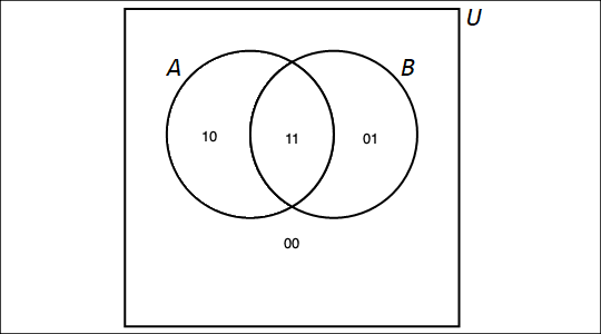
If you had instead three subsets \(A\), \(B\), and \(C\) of the universal set \(U,\) you could partition the universe \(U\) into 8 subsets. In detail, if you have an element \(x \in U\), either \(x \in A\) or \(x \not\in A\), and for each of those possibilities, either \(x \in B\) or \(x \not\in B\), and for each of those possibilities, either \(x \in C\) or \(x \not\in C\). We can apply (twice) the multiplication principle that was first mentioned in chapter 2 to show that there are \(2 \cdot 2 \cdot 2\) possible subsets determined by the Venn diagrams of the 3 sets \(A\), \(B\), and \(C\). Using bitstrings of length 3, we can label these 8 subsets as shown.
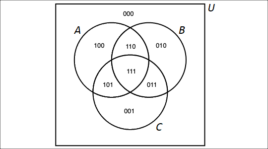
For an integer \(n > 3\), the Venn diagram is less useful for representing the partitioning of the universe created by \(n\) subsets, but we can still reason that there ought to be \(2^{n}\) subsets in the partition, where each of the subsets can be described by a unique bitstring of length \(n\) (We will be able give a formal mathematical proof of this for every positive integer \(n\) later in the textbook after we’ve discussed mathematical induction.)
4.11.1. Disjunctive Normal Form (Set Version)
Suppose you have three sets \(A\), \(B\), and \(C\), and have partitioned the universe \(U\) into the 8 subsets as discussed above. A subset of \(U\) that corresponds to any shading of the Venn diagram can be written as a union of intersections of three sets, with one set chosen from each of the pairs \(\{ A,\,\overline{A} \}\), \(\{ B,\,\overline{B} \}\), and \(\{ C,\,\overline{C} \}\).
As an example, consider the set shown in the image, which has 4 of the 8 regions of the Venn diagram shaded:
-
\(\overline{A} \cap \overline{B} \cap \overline{C}\) which is the region outside of all three sets,
-
\(A \cap \overline{B} \cap \overline{C},\) the region in set \(A\) but in neither \(B\) nor \(C,\)
-
\(\overline{A} \cap B \cap \overline{C},\) the region in set \(B\) but in neither \(A\) nor \(C,\)
-
\(\overline{A} \cap B \cap C,\) the region in both \(B\) and \(C\) but not in \(A.\)
Write the union of these 4 subsets to create an expression that describes the entire shaded region. \[(\overline{A} \cap \overline{B} \cap \overline{C}) \cup (A \cap \overline{B} \cap \overline{C}) \cup (\overline{A} \cap B \cap \overline{C}) \cup (\overline{A} \cap B \cap C)\]
This type of expression is called a disjunctive normal form (or DNF) for the set that it represents. We will see an analog of these in a different context in the chapter on Logic.
The advantage of using the DNF is that you can write out an expression for the shaded subset using a simple algorithm. The DNF may be neither the shortest possible expression nor the most easily understood expression for the shaded part of the Venn diagram, but the DNF is a correct expression for the shaded subset.
4.12. The Principle Of Inclusion-Exclusion (PIE)
In certain application problems, we want to compute the cardinality \(|A \cup B|\) of the union of two given finite sets \(A\) and \(B\). It is tempting to simply add \(|A|\) and \(|B|\), but as the Venn diagram below shows, each element of the intersection \(|A \cap B|\) will be counted twice, once for each bit that is \(1\), if we do so.
The correct relationship between \(|A \cup B|\), \(|A|\), and \(|B|\) is given by \[ |A \cup B| = |A| + |B| - |A \cap B|. \]
Another way to see that this is the correct relationship is to use the partition \(\{ \overline{A} \cap \overline{B},\, \overline{A} \cap B,\,A \cap \overline{B},\,A \cap B \}\) to write
\(| A | = | A \cap \overline{B} | + | A \cap B |\),
\(| B | = | \overline{A} \cap B | + | A \cap B |\), and
\(| A \cup B | = | A \cap \overline{B} | + | A \cap B | + | \overline{A} \cap B |\), so
\(| A | + | B | = | A \cap \overline{B} | + | A \cap B | + | \overline{A} \cap B | + | A \cap B | = | A \cup B | + | A \cap B |\).
If we want to compute the cardinality \(|A \cup B \cup C|\) of the union of three given finite sets \(A\), \(B\), and \(C\), we can again look at the Venn diagram of the partition of \(U\) into 8 sets to see that some of the intersections will be counted one, two, or three times, once for each bit that is \(1\).
We can derive the following formula in much that same way that we did above; in fact, we can just apply the formula we found for two sets to \(| (A \cup B) \cup C |\) and use some of the set identities to help simplify the formula. \[ |A \cup B \cup C| = |A| + |B| + |C| - |A \cap B| - |A \cap C| - |B \cap C| + |A \cap B \cap C|. \]
4.13. Cardinality Of Sets: Infinite Sets
Set \(A\) is called an infinite set if it not a finite set. That is, \(A\) is not the empty set, and for every positive integer \(n\) there is no one-to-one correspondence between \(A\) and \(\{1, 2, \ldots , n \}.\)
Intuitively an infinite set \(A\) is at least as big as the set of positive integers. You may think that \(A\) must have the same size as the set of positive integers, but cardinality is a much more … "interesting" concept for infinite sets, as you will see.
First, we will say that two infinite sets \(A\) and \(B\) have the same cardinality if and only if there is a one-to-one correspondence between the two sets. As an example, the set of positive integers and the set of negative integers have the same cardinality since each nonzero integer \(n\) can be paired with its additive inverse, \(-n.\)
For finite sets, if \(A\) is a proper subset of \(B\) then it must be true that the cardinality of \(A\) is not the same as the cardinality of \(B.\) This fails spectacularly for infinite sets as the next few examples show.
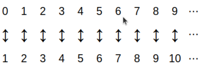
The image shows that there is a one-to-one correspondence between the natural numbers and the positive integers, so these two sets have the same cardinality. But this isn’t so bad, we only have one more number in the set of natural numbers, which is why we can just shift every thing over by 1 in the image.
Notice that this example also suggests why it really does not matter whether we start counting from 1 or 0… we can always "reindex" the counting if necessary.
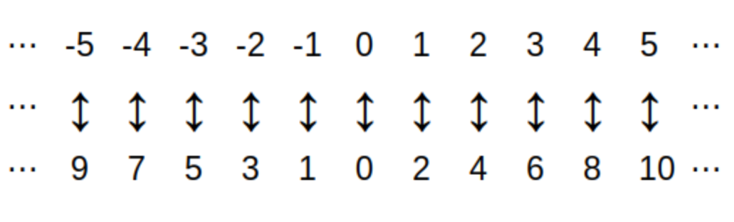
The image shows that there is a one-to-one correspondence between the set of all integers and the natural numbers.
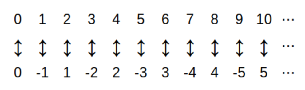
The image shows the inverse of the one-to-one correspondence above, which is a one-to-one correspondence between the set of natural numbers and the set of integers.
These two sets have the same cardinality, which may surprise you since "intuitively" it would seem there should be about twice as many integers as natural numbers. However, this example shows that you can double (roughly) the size of an infinite set and get a new set that has the same cardinality.

This first image, which shows red points plotted in the \(xy\)-plane that have been labeled with natural numbers, suggests a way to define a one-to-one correspondence between the set of ordered pairs of natural numbers, \(\mathbb{N} × \mathbb{N},\) and the set of natural numbers \(\mathbb{N}.\)
Image credit: "Cantor’s Pairing Function" by crh23. The image is dedicated to the public domain under CC0.
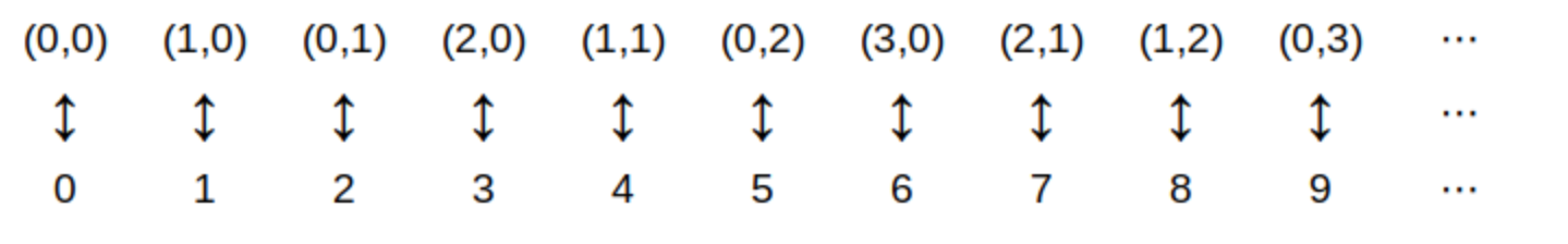 This second image displays the same one-to-one correspondence in tabular form.
In the first image, notice that for each fixed value of the second coordinate \(y \in \mathbb{N},\) the horizontal row of red points of the form \(\{ (x, y) : x \in \mathbb{N} \} = \{ (0, y), (1, y), (2, y), (3, y), \ldots \}\) has the same cardinality as \(\mathbb{N}\) and
that there is one such row for every natural number \(y \in \mathbb{N}.\) That is, the set of rows has the same cardinality as the set \(\mathbb{N},\) and each of the rows has the same cardinality as \(\mathbb{N}.\)
There are, in essence, as many copies of \(\mathbb{N}\) (the rows of red points) as there are elements in \(\mathbb{N},\) and these copies are joined together to form the Cartesian product \(\mathbb{N} × \mathbb{N}\)… but this set still has the same cardinality as \(\mathbb{N}.\)
Notice something else about this example: It shows that each pair of natural numbers can be encoded as a single natural number. In fact, this example can be generalized to show that any element in the set of all finite-length sequences of natural numbers can be encoded uniquely to a natural number (so, for example, the set of all possible finite-length strings of Unicode characters/code points can be encoded to the set of natural numbers, which may or may not be surprising to you.)
You may want to read about triangular numbers to get an idea of how the mapping of ordered pairs to numbers is being done. In the first image, the red points form a "triangle of infinite height" with a vertex at \((0,0)\) and sides lying along the \(x-\) and \(y-\)axes. "Row 0" of the triangle is the single point \((0,0),\) and "row \(n\)" of the triangle is made up of the red points with natural number coordinates \((x,y)\) that add up to \(n\) (that is, \(x+y = n\).)
A proof that this mapping of ordered pairs of natural numbers to individual natural numbers is in fact a one-to-one correspondence will be presented later in the textbook.
So far, every infinite set presented has the same cardinality as \(\mathbb{N}.\)
Maybe all infinite sets have the same cardinality as \(\mathbb{N}?\) Nope!
The next theorem shows that \(\mathcal{P}(\mathbb{N})\) cannot have the same cardinality as \(\mathbb{N}\) so there must be at least two "infinities."
There is no one-to-one correspondence between \(\mathbb{N}\) and \(\mathcal{P}(\mathbb{N}).\)
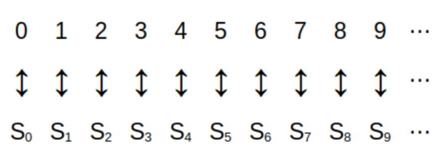 Let’s suppose that we had such a one-to-one correspondence.
As shown in the image, we could represent the one-to-one correspondence by a sequence \(S_0 , S_1 , S_2 , \ldots\) of subsets of \(\mathbb{N},\) which is what the elements of \(\mathcal{P}(\mathbb{N})\) are. In the one-to-one correspondence, every subset of \(\mathbb{N}\) (that is, every element of \(\mathcal{P}(\mathbb{N})\)) appears as one of the \(S_{n}\) in the sequence: Every subset has been paired with a natural number and every natural number has been paired with a subset.
Let’s suppose that we had such a one-to-one correspondence.
As shown in the image, we could represent the one-to-one correspondence by a sequence \(S_0 , S_1 , S_2 , \ldots\) of subsets of \(\mathbb{N},\) which is what the elements of \(\mathcal{P}(\mathbb{N})\) are. In the one-to-one correspondence, every subset of \(\mathbb{N}\) (that is, every element of \(\mathcal{P}(\mathbb{N})\)) appears as one of the \(S_{n}\) in the sequence: Every subset has been paired with a natural number and every natural number has been paired with a subset.Next, define a subset \(M \subseteq \mathbb{N}\) as \[M = \{ n \in \mathbb{N} : n \not\in S_n \}\] That is, \(M\) is defined by the rule that for each natural number \(n,\) we have \(n \in M\) if and only if \(n \not\in S_{n}.\) So, for example, 0 is an element of \(M\) if 0 is not an element of \(S_0,\) but is not an element of \(M\) if 0 is an element of \(S_0.\) Likewise, 1 is an element of \(M\) if 1 is not an element of \(S_1,\) but is not an element of \(M\) if 1 is an element of \(S_1.\) The same is true for each of the natural numbers 2, 3, and so on: The natural number \(n\) is an element of exactly one of the sets \(S_n\) and \(M.\)
Now we show that \(M\) must be missing from the sequence \(S_0 , S_1 , S_2 , \ldots\)
\(M\) cannot be \(S_0\) since one of those sets contains 0 and the other one does not. \(M\) cannot be \(S_1\) since one of those sets contains 1 and the other one does not. The same must be true for each of the natural numbers 2, 3, and so on. So, for every natural number \(n,\) \(n\) is an element of exactly one of the two sets \(S_n\) and \(M,\) which means \(M \neq S_n\) is true for every natural number \(n.\) This means that \(M\) cannot be any of the sets in the sequence… it is missing!
We assumed that every subset is listed in the sequence, but just showed that there is some subset that is not listed in the sequence. Notice that, even if we tried to use a new sequence (for example, insert \(M\) at position 0 and shift all the other subsets over by adding 1 to their subscripts) the diagonal argument could be used to define another subset that is missing from the new sequence. So, every possible sequence of subsets must be missing at least one subset.
Therefore, such a one-to-one correspondence cannot exist.
4.13.1. Countable and Uncountable Sets
Set \(A\) is called countable if
-
\(A\) is a finite set or
-
there is a one-to-one correspondence between \(A\) and \(\mathbb{N}.\) In this case, \(A\) is also called countably infinite.
Set \(A\) is called uncountable if it is not a countable set. That is, \(A\) is infinite and there is no one-to-one correspondence between \(A\) and \(\mathbb{N}.\)
Several examples of countably infinite sets were given in the examples in the preceding subsection:
-
The set of positive integers \(\{ i \in \mathbb{N} \, | \, i > 0 \},\)
-
the set of integers \(\mathbb{Z},\) and
-
the set of ordered pairs of natural numbers, \(\mathbb{N} × \mathbb{N}.\)
On the other hand, the theorem in the preceding subsection shows that \(\mathcal{P}(\mathbb{N})\) is an uncountable set.
Infinite Cardinal Numbers
In advanced mathematics, the concept of "infinite cardinal number" is developed and used to represent the sizes of infinite sets. Mathematicians use these infinite cardinal numbers to make sense of cardinalities like \(|\mathbb{N}|\) and \(|\mathcal{P}(\mathbb{N})|.\) It can be proven that \[|\mathbb{Q}| = |\mathbb{N}|\] \[|\mathbb{N}| < |\mathcal{P}(\mathbb{N})|\] \[|\mathcal{P}(\mathbb{N})| = |\mathbb{R}|\] and that \[\text{for any infinite set } A, |A| < |\mathcal{P}(A)|\] which shows that there must be infinitely-many infinite cardinal numbers.
4.14. Exercises
Remixer’s Note: This section is taken from the original “Discrete Math” book with only minor changes.
-
Consider as universal set, the set of all \(26\), lowercase letters of the English alphabet, \(U=\{a,b,c,…,v,w,x,y,z\}\), and the sets \(A=\{a,b,c,d,e,f,g,h\}\), \(B=\{f,g,h,i,j,k\}\), and \(C=\{x,y,z\}\). For the sets given below:
-
List the sets below using roster form, and
-
Draw Venn Diagrams for each of the sets
-
\(A\cup B\)
-
\(A\cap B\)
-
\(A\cup C\)
-
\(A\cap C\)
-
\(A \setminus B\)
-
\(B \setminus A\)
-
\(A \setminus C\)
-
\(C \setminus A\)
-
\(A\cup C\)
-
\(A\cap C\)
-
\(\overline{A}\)
-
\(\overline{B}\)
-
\(\overline{C}\)
-
\(\overline{B} \cap \overline{C}\)
-
\( (\overline{A} \cap \overline{B}) \cup (\overline{B} \cap \overline{C})\)
-
-
-
Using Venn Diagrams, determine which of the following are equivalent
-
\(A \setminus (A \setminus B)),\)
\(A\cup B,\) and
\(A\cap B\)
-
\(A\cup \overline{A},\)
\(A\cap \overline{A},\)
\(U,\) and
\(\emptyset\)
-
\(\overline{A}\cap \overline{B}, \)
\(\overline{A\cap B},\)
\(\overline{A}\cup \overline{B},\) and
\(\overline{A\cup B}\)
-
\(A\cup (B\cap C),\)
\(A\cap (B\cup C),\)
\((A\cap B)\cup (A\cap C),\) and
\((A\cup B)\cap (A\cup C),\)
-
\(\overline{\overline{A}\cup(C \setminus B) }),\)
\(A\cap (B \cup \overline{C}),\) and
\(A \setminus (C \setminus B)\)
-
-
Write each of the following sets using set builder notation
-
\(\{\ldots, -9, -7, -5, -3, -2, -1, 1, 3, 5, 7, 9, \ldots \}\)
-
\(\{\ldots, -8, -6, -4, -2, 0, 2, 4, 6, 8, 10,\ \ldots \}\)
-
\(\{ 1, 2, 3, 4, 5, 6, 7, 8, 9, 10 \}\)
-
\(\left\{ 1,\frac{1}{2},\frac{1}{3},\frac{1}{4},\frac{1}{5},\ldots \right\}\)
-
\(\{0, 1, 4, 9, 16, 25, 36, 49, \ldots \}\)
-
\(\{\ldots,-10,-6, -2, 2, 6, 10, 14, 18, 22, \ldots \}\)
-
\(\{ 3, 9, 27, 81, 243,\ldots\}\)
-
\(\{ 1, 9, 25, 49, 81, \ldots \}\)
-
-
Write each of the following sets in roster form
-
\(\{x \in \mathbb{R} : |2x+5|=7\}\)
-
\(\{10n : n \in \mathbb{N}\}\)
-
\(\{10n : n \in \mathbb{Z}\}\)
-
\(\left\{2^n : n \in \mathbb{N}\right\}\)
-
\(\left\{2^n : n \in \mathbb{Z}\right\}\)
-
\(\left\{x \in \mathbb{R} : x^2=4\right\}\)
-
\(\left\{x \in \mathbb{R} : x^3=64\right\}\)
-
\(\left\{x \in \mathbb{Z} : x^2=5\right\}\)
-
\(\left\{x \in \mathbb{R} : x^2= -4\right\}\)
-
\(\left\{x \in \mathbb{Z} : |x-5|=3\right\}\)
-
\(\left\{3n+4 : n \in \mathbb{N}\right\}\)
-
\(\left\{3n+4 : n \in \mathbb{Z}\right\}\)
-
\(\left\{i^n : n \in\mathbb{N}\right\}\), where \(i\) is such that \(i^2=-1\) (the imaginary unit).
-
-
Consider the sets \(A=\{1, 3, 5, 7, 9, 11, 13, 15, 17\}\), \(B=\{2, 5, 7, 11\}\), and \(C=\{1, 2, 3\}\),
-
Determine the cardinalities of following sets,
-
\(|A|\)
-
\(|A\cup B|\)
-
\(|A\cap C|\)
-
\(|\mathcal{P}(A)|\)
-
\(|\mathcal{P}(B)|\)
-
\(|\mathcal{P}(C)|\)
-
-
Give the following power sets,
-
\(\mathcal{P}(B)\)
-
\(\mathcal{P}(C)\)
-
-
-
Determine the cardinalities of following sets,
-
\(\{n \in \mathbb{Z} : |n|\leq 10\}\)
-
\(\{A,B, \emptyset,\{2,5,6\}\}\)
-
\(\{\{A,B\},\{\},\{\{2,5,6\}\},\{\{2,5,6\},C\},\{A,B,C\}\}\)
-
\(\{\{\{A,B\},\emptyset,\{\{2,5,6\},C\},\{A,B,C\}\}\}\)
-
-
Consider the sets, \(B=\{0, 1\}\), \( S=\{spring, summer, fall, winter\}\), and \(C=\{ a, b, c, d,e\}\). For each of the following sets:
-
Determine the following Cartesian products.
-
Calculate the cardinality of each Cartesian product.
-
\(B \times S\)
-
\(S \times B\)
-
\(B \times C\)
-
\(C \times B\)
-
\(B \times B \times B \times B\)
-
\(S \times B \times B\)
-
-
-
Determine the following power sets,
-
\(\mathcal{P}(\{Alabama, Georgia, Florida, Louisiana\} )\)
-
\(\mathcal{P}(\emptyset )\)
-
\(\mathcal{P}(\{\emptyset\} )\)
-
\(\mathcal{P}(\{Alabama \} )\)
-
\(\mathcal{P}(\{Alabama, Georgia, Florida \} )\)
-
\(\mathcal{P}(\{\{Alabama, Georgia \}, \{Florida \} \} )\)
-
-
Write the shaded regions in each of the following Venn diagrams using set notation.
-
Determine if each of the following are true or false. Explain your reasoning.
-
\(\{7,4,6,2,11,3,5\}\subseteq \{1,2,3,4,5,6,7,8,9,10,11,12,13\}\)
-
\(\{1,2,3,4,5,6,7,8,9,10,11,12,13\}\subseteq \{7,4,6,2,11,3,5\}\)
-
\(\{7,4,6,2,11,3,5\}\subseteq \{7,4,6,2,11,3,5\}\)
-
\(\{3,8\}\nsubseteq \{7,4,6,2,11,3,5\}\)
-
\( \{3n+4 : n \in \mathbb{N}\} \nsubseteq \mathbb{Z}\)
-
\(\mathbb{N}\subseteq \mathbb{Z}\subseteq \mathbb{Q}\subseteq \mathbb{R}\)
-
\(\{x \in \mathbb{R} : |x|<3\}\subseteq \{x \in \mathbb{R} \, | \, |x|<5\}\)
-
\(\{x \in \mathbb{R} : |x|>3\}\subseteq \{x \in \mathbb{R} \, | \, |x|>5\}\)
-
5. Logic
CAUTION - CHAPTER UNDER CONSTRUCTION!
NOTICE: If you are NOT enrolled in the CSC 230 course that I teach at SFSU, you probably are looking for the “public version” of the book, which I only update between semesters. The version you are looking at now is the “CSC230 version” of the book, which I will be updating throughout the semester.
This chapter was last updated on September 23, 2025.
Edited section on logic circuits.
Logic is the study of reasoning. Logic is used to create, analyze, and validate arguments, where an argument is a finite sequence of statements that ends with a conclusion based on inferences made from earlier statements in the argument.
Among the applications of logic to computer science are design of electronic circuits and validation of algorithms and programs.
Key terms and concepts covered in this chapter:
-
Propositional logic (also called "propositional calculus")
-
Logical operators (also called "logical connectives")
-
Negation ("not")
-
Conjunction ("and")
-
Disjunction ("or")
-
Conditional ("implication")
-
The converse, inverse, and contrapositive of a conditional
-
-
Biconditional ("if and only if," abbreviated as "iff")
-
-
Truth tables
-
Well-formed formulas
-
Satisfiability, tautology, and contradiction
-
Normal forms (conjunctive and disjunctive)
-
-
Predicate logic
-
Predicates as "statement-valued functions"
-
Quantification of Predicates
-
Universal quantifier
-
Existential quantifier
-
-
-
To be added to this chapter after May 23, 2025:
-
Limitations of propositional and predicate logic (e.g., expressiveness issues)
-
Boolean algebra and Boolean circuits
-
5.1. Propositional Logic
A proposition is a statement that declares a fact that is either True or False (but not both!)
Propositional logic consists of a set of formal rules for combining propositions in order to derive new propositions.
A goal of propositional logic is to have a method for creating valid arguments that are sequences of propositions, where the correctness and validity of the argument is based solely on the propositions' truth values (True and False), ignoring the actual content of the propositions. Compare this to doing algebra: You can write \(2 (x + 3 y) = 2x + 6y\) because it is a correct and valid step to distribute multiplication over addition. You can do the algebra and ignore the specific numerical values (the "numerical content") that \(x\) and \(y\) stand for.
In propositional logic, it is traditional to use propositional variables such as p, q, and r to stand for the possible assignments of truth values to propositions; often, the propositional variables themselves are referred to as the propositions. Again, compare this to the algebraic example where you can treat \(x\) and \(y\) as numbers even though they are actually variables that stand for numbers.
What is the advantage of using symbols? A long time ago, philosophers discovered that is easier to follow lines of reasoning by putting our thoughts into symbols. This was an important step in the eventual development of modern technological society and, in particular, electronic computers. Before a computer can do its work, humans need to put our thoughts into them; however, a spoken language like English can be too difficult to use because many different phrases can represent the same logical statements.
You can build compound propositions (also called "propositional functions") from simpler propositions. For example, in the preceding example, the compound propostion "if p then q" was introduced as a new proposition built from the propositional variables p and q. In the next section, you will learn how to represent compound propositions using symbols.
5.2. Logical Operations and Truth Tables
In this section, compound propostions will be represented by using propositional variables and logical operator symbols (also called "logical operations" or "logical connectives") Once again, you can compare this to how numerical and algebraic relationships can be represented in symbols using algebraic expressions built with the usual arithmetic operator symbols with variables and numerals.
|
In Python, we use \(\texttt{Boolean}\) variables to represent propositions and define functions for each compound proposition. Each compound proposition can implemented using the \(\texttt{Boolean}\) operations \(\texttt{not}\), \(\texttt{and}\), and \(\texttt{or}\) discussed in the section Operators and Expressions in the chapter "Appendix: An Introduction to Python". |
A truth table can be used to display the truth values of a compound proposition that is built from propositional variables and logical operators. A truth table is created with rows representing all possible interpretations of the propositional variables, that is, all possible assignments of truth values to the propositional variables. Each column of a truth table displays the truth values for either one of the propositional variables or a compound proposition built up from propositional variables and/or simpler compound propositions. As an analogy, think of how a table can be used to display the numerical input and output values of a function represented by an algebraic expression.
The most commonly-used logical operators are described in the rest of this section.
5.2.1. Negation
"I am not an astronaut."
The negation of a proposition \(p\), denoted in mathematics by \(\neg p\) and
read as "not \(p\)", is the proposition
"It is not the case that \(p\)".
The proposition \(\neg p\) has the opposite truth value to \(p.\)
Other textbooks and sources may use \(\overline{p}\) or \(\sim \! p\) to represent \(\neg p.\)
| \(p\) | \(\neg p\) |
|---|---|
True |
False |
False |
True |
For example, the negation of the proposition "Today is Friday." would be
"It is not the case that today is Friday." or more succinctly "Today is not Friday."
For a proposition \(p,\) exactly one of \(p\) and \(\neg p\) is True and exactly one is False. Two propositions can be contrary (that is, they could not both be True) without being negations of each other: As an example, both of the propositions "Today is Friday." and "Today is Saturday." could be False, so "Today is Saturday." is not the negation of "Today is Friday."
Notice that the two propositions \(p\) and \(\neg (\neg p)\) must always have the same truth value (You can see this by inserting a column for \(\neg (\neg p)\) in the truth table shown earlier in this subsection.)
| In the first few truth tables in this chapter, "True" and "False" are spelled out, but it is more often the case that these words are abbreviated to their first letters, "T" and "F" in truth tables. |
5.2.2. Conjunction
"I am a rock and I am an island."
Let \(p\) and \(q\) be propositions. The conjunction of \(p\) and \(q\), denoted in mathematics by \(p \land q\) and read as "\(p\) and \(q\)", is True when both \(p\) and \(q\) are True and is False otherwise.
| \(p\) | \(q\) | \(p \land q\) |
|---|---|---|
True |
True |
True |
True |
False |
False |
False |
True |
False |
False |
False |
False |
Notice that the two propositions \(p \land q\) and \(q \land p\) always have the same truth value.
5.2.3. Disjunction
"They studied hard or they are extremely bright."
Let \(p\) and \(q\) be propositions. The disjunction of \(p\) and \(q\), denoted in mathematics by \(p \lor q\) and read as "\(p\) or \(q\)", is True when at least one of \(p\) and \(q\) are True and is False otherwise.
| \(p\) | \(q\) | \(p \lor q\) |
|---|---|---|
True |
True |
True |
True |
False |
True |
False |
True |
True |
False |
False |
False |
Notice that the two propositions \(p \lor q\) and \(q \lor p\) always have the same truth value.
5.2.4. Conditional
"If you get a 100 on the final exam, then you earn an A in the class."
Let \(p\) and \(q\) be propositions. The conditional statement \(p \rightarrow q\), read as "if p then q", "p implies q", or, more formally, "the conditional with hypothesis p and conclusion q", is the proposition that is False when p is True and q is False, and True otherwise. The conditional statement \(p \rightarrow q\) is also called "the implication \(p \rightarrow q\)".
The conditional \(p \rightarrow q\) can also be denoted by \(p \Rightarrow q\) or \(p \implies q.\) In addition, there are many other ways to express the conditional \(p \rightarrow q\) in English, two of which are "p only if q" and "q if p".
| \(p\) | \(q\) | \(p \rightarrow q\) |
|---|---|---|
True |
True |
True |
True |
False |
False |
False |
True |
True |
False |
False |
True |
|
|
The Converse, Contrapositive and Inverse of a Conditional Statement
Given propositions p and q, we can form three additional compound propositions that are related to the conditional \(p \rightarrow q\):
-
\(q \rightarrow p\), called the converse of \(p \rightarrow q\)
-
\( \neg q \rightarrow \neg p\), called the contrapositive of \(p \rightarrow q\)
-
\( \neg p \rightarrow \neg q\), called the inverse of \(p \rightarrow q\)
The extended truth table for the conditional and the three related propositions is shown below.
| \(p\) | \(q\) | \(p \rightarrow q\) (conditional) | \(q \rightarrow p \) (converse) | \( \neg q \rightarrow \neg p\) (contrapositive) | \( \neg p \rightarrow \neg q\) (inverse) |
|---|---|---|---|---|---|
True |
True |
True |
True |
True |
True |
True |
False |
False |
True |
False |
True |
False |
True |
True |
False |
True |
False |
False |
False |
True |
True |
True |
True |
|
From the truth table it can be seen that
|
In the section on logically equivalent propositions we will discuss the bullet points in the preceding note in more detail.
The next example illustrates these four propositions.
5.2.5. Biconditional
"It is raining outside if and only if it is a cloudy day."
Let \(p\) and \(q\) be propositions. The biconditional \(p \leftrightarrow q\), read as "p if and only if q", is the proposition that is True when p and q have the same truth value, and False otherwise. The biconditional is also called "the bi-implication". Note that \(p \leftrightarrow q\) can also be denoted by \(p \Leftrightarrow q\) or \(p \iff q.\)
| \(p\) | \(q\) | \(p \leftrightarrow q\) |
|---|---|---|
True |
True |
True |
True |
False |
False |
False |
True |
False |
False |
False |
True |
You can use a truth table to show that two propositions \(p \leftrightarrow q\) and \(q \leftrightarrow p\) always have the same truth value.
|
The biconditional \(p \leftrightarrow q\) is read as "p if and only if q" because it has the same truth table as the conjunction of the two conditionals "p if q" (that is, \(q \rightarrow p\)) and "p only if q" (that is, \(p \rightarrow q\)). |
It is important to contrast the conditional with the biconditional. Consider the conditional example "If you get a 100 on the final exam, then you earn an A in the class." This means that when you get a 100 on the final you also get an A in the class. The conditional represents a one-way contract: You earn an A in the class if you get a 100 on the final exam. There is nothing said about the result (the grade you earn in the class) if you do NOT meet the condition (get a 100 on the final exam).
As a biconditional the example would say "You get a 100 on the final exam if and only if you earn an A in the class." This becomes a two-way contract: You earn an A in the class if you get a 100 on the final, but you do not earn an A in the class if you do not get a 100 on the final.
5.2.6. Other Compound Propositions
The negation, disjunction, conjunction, conditional, and biconditional are the most commonly-used logical operators for forming compound propostions and will be the ones used throughout the rest of this chapter. However, there are at least three others you should know about.
Exclusive Disjunction
"I took either 2 Advil or 2 Tylenol."
Let \(p\) and \(q\) be propositions. The exclusive disjunction of \(p\) and \(q\) (also known as xor), denoted in mathematics by \(p \oplus q\), is True when exactly one of \(p\) and \(q\) are True and False otherwise.
| \(p\) | \(q\) | \(p \oplus q\) |
|---|---|---|
True |
True |
False |
True |
False |
True |
False |
True |
True |
False |
False |
False |
Notice that the two propositions \(p \oplus q\) and \(q \oplus p\) always have the same truth value.
The NAND and NOR Operators
The NAND and NOR operators correspond to two important digital logic gates used in electronic devices.
NAND
"An onion is not both a fruit and a vegetable."
Let \(p\) and \(q\) be propositions. In this textbook, the NAND of \(p\) and \(q\) is denoted by \(p \uparrow q\) and is False when both \(p\) and \(q\) are True and is True otherwise. That is, the NAND is the negation of \(p \land q\) - think of NAND as "Not AND."
| \(p\) | \(q\) | \(p \uparrow q\) |
|---|---|---|
True |
True |
False |
True |
False |
True |
False |
True |
True |
False |
False |
True |
Notice that the two propositions \(p \uparrow q\) and \(q \uparrow p\) always have the same truth value.
NOR
"This pen’s ink is neither red nor blue."
Let \(p\) and \(q\) be propositions. In this textbook, the NOR of \(p\) and \(q\) is denoted by \(p \downarrow q\) and is True when both of \(p\) and \(q\) are False and is False otherwise. The NOR is also referred to as "joint denial" since it is True exactly when neither \(p\) nor \(q\) is True. That is, the NOR is the negation of \(p \lor q.\)
| \(p\) | \(q\) | \(p \downarrow q\) |
|---|---|---|
True |
True |
False |
True |
False |
False |
False |
True |
False |
False |
False |
True |
Notice that the two propositions \(p \downarrow q\) and \(q \downarrow p\) always have the same truth value.
5.2.7. Well-Formed Formulae and Operator Precedence (Order Of Operations)
A well-formed formula (or wff for short) is a string of symbols that represents a compound propsition.
Here is a recursive definition of wff:
-
A propositional variable is a well-formed formula.
-
If \(\alpha\) ("alpha") and \(\beta\) ("beta") are well-formed formulas, then the following are also well-formed formulas:
-
\(\left( \neg \alpha \right)\)
-
\(\left( \alpha \land \beta \right)\)
-
\(\left( \alpha \lor \beta \right)\)
-
\(\left( \alpha \rightarrow \beta \right)\)
-
\(\left( \alpha \leftrightarrow \beta \right)\)
-
The definition of wff allows you or, even better, a computer to analyze any string of symbols to determine whether the string of symbols is a wff. For example, \((p \land q \lor r)\) isn’t a wff but both \((p \land (q \lor r))\) and \(((p \land q) \lor r)\) are wffs. You could write code to implement an algorithm to validate a string as a wff.
It can be shown that every compound proposition can be represented by at least one wff. However, a wff may be difficult to read quickly if it contains many parentheses. As an example, it is not easy to read \(( (p \rightarrow q) \lor ( (\neg r) \land (s \leftrightarrow t) ) )\). For this reason, we can introduce operator precedence rules that allow us to eliminate some of the parentheses.
To evaluate a compound proposition, we start by evaluating
-
all expressions enclosed in parentheses from left to right, then
-
all negations from left to right, then
-
all conjunctions from left to right, then
-
all disjunctions from left to right, then
-
all conditionals from left to right, and finally
-
all biconditionals from left to right.
This allows us to drop some parentheses from a wff that represents a compound proposition.
For example, the compound proposition \(\neg p \lor q \land r \rightarrow s\) represents the same proposition as the wff \((((\neg p) \lor (q \land r)) \rightarrow s)\). At least some of the parentheses must be used if you want to represent a different proposition such as \((\neg p \lor q) \land (r \rightarrow s)\).
5.2.8. Truth Tables of Compound Propositions
To compute the truth values of a longer compound proposition or wff by hand, it can be useful to break up the proposition or wff into the smaller propositions or wffs that it was built from.
When creating your own truth table it is crucial to be systematic about ensuring you have all possible truth values for each of the simple propositions. Each simple proposition has two possible truth values, so the number of rows in the table should be \(2^n\) where \(n\) is the number of propositions (Do you recall why the number of rows must be \(2^n\)?) You should also consider breaking complex propositions into smaller pieces.
5.3. Logically Equivalent Propositions
Recall that an interpretation of a proposition is an assignment of truth values to the propositional variables.
Two propositions are considered logically equivalent (or simply equivalent) if they have the same truth values for every possible interpretation. It is often easiest to see this by constructing a truth table for the two propositions and comparing.
We use the symbol \(\equiv\) to denote that two propositions are logically equivalent. So in the preceding example, we would write \(\neg p \lor q \equiv p\rightarrow q\).
| \(\equiv\) is NOT a logical operator used to build compound propositions, but instead is used to say that two propositions are logically equivalent. This is similar to how \(=\) is used in arithmetic: We can write \(2 + 2 = 5 - 1\) to say that \(2 + 2\) and \(5 - 1\) are numerically equivalent, but we don’t use the \(=\) sign as an arithmetic operator to actually do any arithmetic. |
| Saying that two propositions p and q are logically equivalent is the same as saying that the biconditional compound proposition \(p \leftrightarrow q\) is always True. |
5.3.1. Tautologies, Contradictions and Contingencies
A proposition is a tautology if its truth value is always True. That is, a tautology is True for every possible interpretation of its propositional variables.
A proposition is called satisfiable if there is at least one interpretation for which the proposition is True.
A proposition is unsatisfiable if there is no interpretation for which the proposition is True.
A proposition is a contradiction if its truth value is always False. That is, a contradiction is False for every possible interpretation of its propositional variables. This is just another way of saying that it is unsatisfiable.
A proposition that is neither a tautology nor a contradiction is said to be a contingency since its truth value can be either True or False, contingent on the truth value assigned to its propositional variables.
The two compound propositions in the previous example are so important that they have their own names,
5.3.2. De Morgan’s Laws
Two important logical equivalences are De Morgan’s Law. These describe how to "distribute" the \(\neg\) operator across the \(\land\) and \(\lor\) operators.
De Morgan’s Laws can be verified by creating truth tables for \(\neg (p \land q) \leftrightarrow \neg p \lor \neg q\) and \(\neg (p \lor q) \leftrightarrow \neg p \land \neg q\) to show that these propositions are True for every interpretation of \(p\) and \(q\).
5.3.3. Some Other Logical Equivalencies
Here is a collection of additional equivalencies of compound propositions. Each of these can be verified by constructing a truth table to show that the biconditional of the left-hand side and the right-hand side of the logical equivalence is true for all interpretations of the propositional variables.
Double Negation: \[ p \equiv \neg (\neg p) \]
Commutative laws: \[ p \lor q \equiv q \lor p \] \[ p \land q \equiv q \land p \]
Associative laws: \[ p \lor (q \lor r) \equiv (p \lor q) \lor r \] \[ p \land (q \land r) \equiv (p \land q) \land r \]
Distributive laws: \[ p \lor (q \land r) \equiv (p \lor q) \land (p \lor r) \] \[ p \land (q \lor r) \equiv (p \land q) \lor (p \land r) \]
5.3.4. Disjunctive Normal Form (DNF)
It is traditional to focus on negation \(\neg\), conjunction \(\land\), and disjunction \(\lor\) as the three primary logical operations. This is because any compound proposition can be rewritten in terms of these three operations and the propositional variables present in the original compound proposition.
One way to justify this is by using an expression in disjunctive normal form (DNF), which is a disjunction of one or more conjunctions, where only one of the conjunctions can be true for any interpretation of the propositional variables. This description should become clearer after reading the following example.
5.3.5. Conjunctive Normal Form (CNF)
In some applications of propositional logic, it is more useful to find a logically equivalent expression for a given proposition that is written as a conjunction of several disjunctions. This conjunctive normal form (CNF) can be constructed as shown in the following example.
Here is a website that allows you to build the DNF and CNF for a given propositional function.
5.3.6. Functional Completeness
A set \(S\) of logical operators is called functionally complete if every compound proposition is logically equivalent to a compound proposition involving only operators that are members of \(S.\)
The importance of the NAND and NOR in electronic circuits arises from the following theorem.
5.4. Predicates and Quantifiers
Up to this point, most of our propositions have been of the form "Sarah earned a B.S. in Computer Science" - the proposition describes a single individual constant (in this case, "Sarah.")
However, we often need to discuss an entire category of individuals at once, which is equivalent to replacing the constant "Sarah" by a variable. We will discuss this idea in this section.
5.4.1. Predicates
A predicate is a statement that includes one or more variables such that when values are assigned to the variables the predicate becomes a proposition.
Predicates are denoted as \(P(x)\) or \(Q(x,y)\) where \(P\) and \(Q\) represent the statements and \(x\) and \(y\) are variables. After a value is assigned to each variable, the predicate becomes a proposition which has a truth value. That is, we "evaluate" a predicate by substituting inputs into the variables and get a proposition as the output.
5.4.2. Quantifiers
Consider the statements
-
For all integers \(x\), \(x^2\geq 0\).
-
Some student in the class has a birthday in July.
Each of these statements considers a proposition over an entire population or set, called the domain, and
describes whether at least one element, or all of the elements
in the
domain
satisfy the proposition.
There are two
commonly-used
quantifiers, the universal quantifier and the existential quantifier.
The domain is also called the domain of discourse or the universe of discourse.
The Universal Quantifier, \(\forall,\) represents the statement "for all", "for every", "for each". When it comes before a statement, it means that statement is true for all values in the domain.
The Existential Quantifier, \(\exists,\) represents the statement "there exists", "for some", "at least one". When it comes before a statement, it means the statement is true for at least one value in the domain.
Recall the previous example statements:
-
For all integers \(x\), \(x^2 \geq 0\).
Let \(P(x)\) be the predicate "\(x^2 \geq 0\)". Then we write the statement as \(\forall x P(x)\), where the domain is the set of all integers. This quantified statement will be true since anytime you square a nonzero integer it is positive and \(0^2=0\).
-
Some student in the class has a birthday in July.
Let \(Q(s)\) be the predicate "student \(s\) has a birthday in July". Then we write the statement as \(\exists s Q(s)\), where the domain is the set of all students in the class. This statement will be true as long as at least one student in the class has a birthday in July. It will be false, otherwise.
5.4.3. Negation of Quantifiers
It is important to consider the negation of a quantified expression.
-
"Every student in this class has taken Programming Fundamentals."
This is a universally quantified statement and can be expressed as \(\forall x P(x)\) where \(P(x)\) is the statement "\(x\) has taken Programming Fundamentals" and the domain consists of all the students in this class. The negation of the statement would be "It is not true that every student in this has taken Programming Fundamentals." Equivalently,
-
"There is a student in this class who has NOT taken Programming Fundamentals."
This is an existentially quantified statement expressed as \(\exists x \neg P(x)\).
This demonstrates that the negation of a universally quantified statement is an existential statement. In symbols, we have \(\neg \forall x P(x)\equiv \exists x \neg P(x)\).
Similarly, the negation of an existential statement is a universal statement. \(\neg \exists x P(x) \equiv \forall x \neg P(x)\).
The predicate of a quantified statement could be a compound statement. For instance,
-
Some dogs are big and fluffy.
This is written as \(\exists x (B(x) \land F(x))\) where \(B(x)\) is the proposition "\(x\) is big." and \(F(x)\) is the proposition "\(x\) is fluffy." and the domain is dogs. Negating this statement would give
\(\neg \exists x (B(x) \land F(x)) \equiv \forall x \neg (B(x) \land F(x)) \equiv \forall x (\neg B(x) \lor \neg F(x))\)
In words,
-
All dogs are not big or not fluffy.
5.4.4. Nested Quantifiers
There are times it will take more than one quantifier to express a statement.
-
For all integers \(x\), there exists an integer \(y\), such that \(x+y=0\).
This statement contains both a universal and an existential quantifier. \(\forall x \exists y S(x,y)\) where \(x\) and \(y\) are integers and \(S(x,y)\) is the proposition \(x+y=0\). This statement means, if you have any integer \(x\) (for instance \(x=5\)) then you can find an integer \(y\) (for instance \(y=-5\)) such that \(x+y=0\).
The order of the quantifiers matters. \(\exists x \forall y S(x,y)\) would be
-
There exists an integer \(x\), such that for all integers \(y\), \(x+y=0\).
Note that in this statement you find an integer \(x\) so that when you add any integer \(y\) to it you always get 0.
The first statement, for all integers \(x\), there exists an integer \(y\) such that \(x+y=0\), is true. For any integer \(x\) you could choose \(y=-x\) and \(x+y=x+(-x)=0\). While the second statement, there exists an integer \(x\), such that for all integers \(y\), \(x+y=0\), is false.
To negate nested quantifiers, repeatedly apply De Morgan’s Laws of negating a quantifier and a predicate.
Namely, \(\neg \forall x P(x) \equiv \exists x \neg P(x)\) and \(\neg \exists x P(x) \equiv \forall x \neg P(x)\).
5.5. Applications of Logic
Remixer’s Note: This section is taken from the original “Discrete Math” book with minor edits to include base-two notation and a link to the NANDgame website.
In this section we consider two applications of logic to information technology and computer science. The first involves bitwise operations, and the second designing and analyzing logic circuits.
5.5.1. Bitwise operations
A bitwise operation is a Boolean operation that operates on the individual bits (\(0s\), or \(1s\)) of the operand(s) and are summarized
We summarize the truth tables for the bitwise boolean operators.
| \(p\) | \(q\) | \(AND\) & | \( \ OR\ | \) | \(XOR\) \({}^{\wedge}\) | \(IF\) \(\Rightarrow\) | \(IFF\) \(\Leftrightarrow\) |
|---|---|---|---|---|---|---|
1 |
1 |
1 |
1 |
0 |
1 |
1 |
1 |
0 |
0 |
1 |
1 |
0 |
0 |
0 |
1 |
0 |
1 |
1 |
1 |
0 |
0 |
0 |
0 |
0 |
0 |
1 |
1 |
5.5.2. Logic Circuits
Logic circuits are important in designing the arithmetic and logic units of a computer processor.
Consider the problem of adding two \(8\)-bit numbers in binary.
In binary, \((0)_2 + (0)_2 = (0)_2\) and \((0)_2 + (1)_2 = (1)_2 + (0)_2 = (1)_2\), but as in decimal addition, \((1)_2 + (1)_2 = (10)_2\) requires a carry, that is, the "sum bit" is \(0\) with a "carry bit" of \(1\) to the next significant column on the left.
Note: The bits are enclosed in parentheses which are followed by the subscript \(_2\) to emphasize that binary notation, not decimal notation, is being used. This notation is covered in much more detail in the Number Bases chapter.
Thinking then of adding a specific column of two binary digits, say \(A\) and \(B\), involves as input the bits \(A, B\) and the carry in from the previous column say \(C_{in}\). The output will be the sum \(S\) and the carry out to the next column, say \(C_{out}\). These are the basic components of what is called a binary adder.
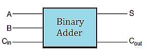
The logic table for binary addition based on the digital inputs \(A, B, C_{in}\), and digital outputs \(S\) and \(C_{out}\) is summarized in the table.
| \(A\) | \(B\) | \(C_{in}\) | \(\mathbf{S}\) | \(\mathbf{C_{out}}\) |
|---|---|---|---|---|
1 |
1 |
1 |
\(\mathbf{1}\) |
\(\mathbf{1}\) |
1 |
1 |
0 |
\(\mathbf{0}\) |
\(\mathbf{1}\) |
1 |
0 |
1 |
\(\mathbf{0}\) |
\(\mathbf{1}\) |
1 |
0 |
0 |
\(\mathbf{1}\) |
\(\mathbf{0}\) |
0 |
1 |
1 |
\(\mathbf{0}\) |
\(\mathbf{1}\) |
0 |
1 |
0 |
\(\mathbf{1}\) |
\(\mathbf{0}\) |
0 |
0 |
1 |
\(\mathbf{1}\) |
\(\mathbf{0}\) |
0 |
0 |
0 |
\(\mathbf{0}\) |
\(\mathbf{0}\) |
You can write logically equivalent expressions for \(S\) and \(C_{out}\) by first writing expressions in Disjucntive Normal Form and then simplifying those expressions using some of the other logical equivalences listed earlier in the chapter: \[S \equiv \left(\sim A\land \sim B\land C_{in}\right)\lor \left(\sim A\land B\land \sim C_{in}\right)\lor \left(A\land \sim B\land \sim C_{in}\right)\lor \left(A\land B\land C_{in}\right) \] \[ C_{out} \equiv (A\land B)\lor \left(B\land C_{in}\right)\lor \left(A\land C_{in}\right)\]
Implementing these logical outputs based on the inputs \((A,B, C_{in})\), is through the use of electronic circuits called logic gates.
The basic logic gates, are the Inverter or Not gate, the And gate, the Or gate and the Xor gate. The graphical representation for each is shown below.
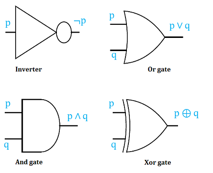
We end this section by first analyzing logic circuits to give their outputs in terms of their input variables, and then, constructing logic circuits based on logical statements.
Determine the output of the following logic circuit in terms of the input variables, \(p, q\), and \(r\).
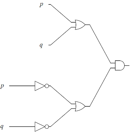
Proceeding left to right, determine the output of the leftmost gates first using the basic gate outputs.
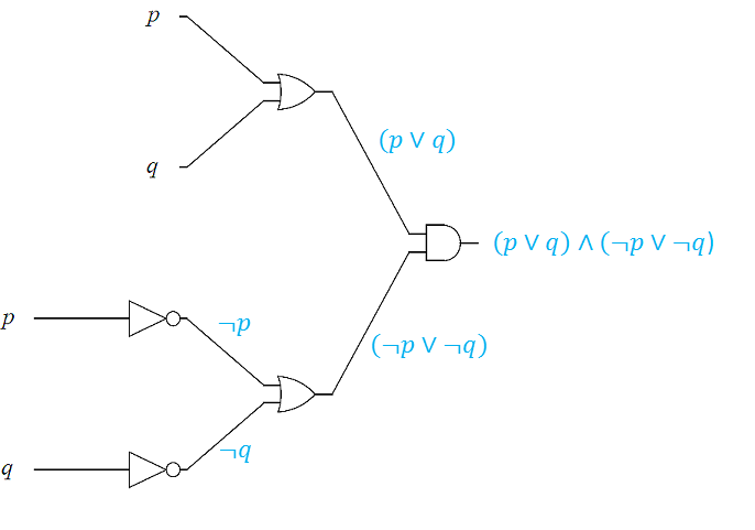
The output of the logic circuit is \( ( p \lor q)\land ( \neg p \lor \neg q)\)
In the next two examples, we design logic circuits based on logical propositions. The idea is to work backward using order of operations from the right to the left.
Design a logic circuit for \((p\vee\lnot\ q)\land\lnot\ p\).
Working backwards from right to left we have the following sequence of gates
1) An AND gate \((p\vee\lnot\ q)\underline{\land} \lnot\ p\).
2) The inputs to the AND gate are \((p\vee\lnot\ q)\) and \(\lnot\ p\).
3) These inputs come from the output of an INVERTER, for \(\underline{\lnot}\ p\) and an OR gate \((p \underline{\vee}\lnot\ q)\).
4) There are two inputs to the OR gate \((p \underline{\vee}\lnot\ q)\), being \(p\), and the output of an INVERTER, \(\underline{\lnot} q\).
Putting these now in left to right order we obtain the following logic circuit.
Design a logic circuit for \(r\land (p\lor (r\land \neg q))\).
Working backwards from right to left we have the following sequence of gates
1) An AND gate \(r\underline{\land} (p\lor (r\land \neg q))\).
2) The inputs to the AND gate are \(r\) and \(p\lor (r\land \neg q)\).
3) The input, \(p\lor (r\land \neg q)\), comes from the output of an OR gate for \(p \underline{\lor} (r\land \neg q)\).
4) The inputs to the OR gate, \(p \underline{\lor} (r\land \neg q)\), are \(p\) and \((r\land \neg q)\), which is an AND gate.
5) The inputs to the AND, gate, \(r \underline{\land} \neg q\), are \(r\) and the output of an INVERTER, \(\underline{\neg} q\).
Putting these now in left to right order we obtain the following logic circuit.
5.6. Exercises
Remixer’s Note: This section is taken from the original “Discrete Math” book with no changes.
-
Which of these statements are propositions? Explain your reasoning
-
Is Atlanta the capital of Georgia?
-
All birds fly
-
\(2\ \times\ \ 3\ =\ 5\)
-
\(5\ +\ 7\ =\ 7+5\)
-
\(x\ +\ 2\ =\ 11\)
-
Answer this question.
-
The rain in Spain
-
-
Construct truth tables for,
-
\(a\vee b\Rightarrow\lnot b\)
-
\((a\vee\lnot b)\ \Leftrightarrow\ a\)
-
\((a\Rightarrow b)\ \bigwedge\ (b\ \bigwedge\ \lnot c)\)
-
\((a\ \bigvee\ b)\ \Rightarrow\ (\ \lnot c\ \bigvee\ a)\)
-
\((a\ \bigvee\ b)\ \bigwedge\ (c\ \bigvee\lnot d\ )\)
-
\((\lnot c\ \bigwedge\ \ b)\ \bigvee\ \ (a\Rightarrow\ \lnot d\ )\)
-
-
Using truth tables, determine if each of the following is a tautology, contradiction, or neither (conditional)
-
\(\neg ((a\lor b)\lor (\neg a\land \neg b))\)
-
\(\left(\left(a\vee b\right)\land\lnot a\right)\Rightarrow b\)
-
\(\left(\left(a\vee b\right)\land a\right)\Rightarrow b\)
-
\(p\land r)\lor (\neg p\land \neg r)\)
-
\(\neg ((p\lor q)\lor (\neg p\land (\neg q\lor r)))\)
-
\(\neg (p\land q)\lor (q\lor r)\)
-
-
Using truth tables determine which of the following are equivalent
-
\(\left(p\Rightarrow q\right)\Rightarrow r\),
\(\left(p\land\lnot q\right)\vee r,\) and
\(\left(p\land\lnot q\right)\land r\)
-
\((a\lor b)\land c,\)
\((c\land a)\lor (c\land b),\) and
\(\neg ((\neg a\land \neg b)\lor \neg c)\)
-
-
Let \(C(x)\) be the statement "\(x\) has visited Canada." where the domain consists of the students at GGC. Express each of the quantifications in English.
-
\(\exists x C(x)\)
-
\(\forall x C(x)\)
-
How would you determine whether each of these statements is true or false?
-
-
Determine the truth value of each of these statements if the domain for all variables, \(m , n\) is the set of all integers, \(\mathbb{Z}\), explaining your reasoning.
-
\(\forall n:\left(n^2\geq 1\right)\)
-
\(\forall n:\left(n^2\geq 0\right)\)
-
\(\ \exists\ n:(n^2=3)\)
-
\(\ \exists\ m\forall\ n:(m+n=n-m)\)
-
\(\forall\ n\exists\ m:\ (n\cdot\ m=m)\)
-
\(\ \exists\ n\forall\ m:\ (n\cdot\ m=m)\)
-
\(\ \exists\ n\forall\ m:\ (n\cdot\ m=n)\)
-
-
Consider each of the compound propositions. (i) Translate each using logical symbols and letters, stating what each letter represents, (ii) Negate each using plain English sentences, and (iii) Translate the negated statements using logical symbols and quantifiers.
-
If it snows today, then I will go skiing tomorrow.
-
Mei walks or takes the bus to class.
-
Every person in this class understands mathematical induction.
-
In every mathematics class there is some student who falls asleep during lectures.
-
There is a building on the campus of some college in the United states in which every room is painted white.
-
-
Let \(p\), be the proposition ”My bicycle needs a tire replaced,” \(q\), be the proposition ”I will go cycling”, and, \(r\), be the proposition ”Rain is in the forecast.”
-
Express each of these compound propositions using plain English sentences.
-
\(\neg p\vee q\)
-
\(\neg p\Rightarrow \neg q\)
-
\((\neg p\wedge r)\Rightarrow q\)
-
\((\neg p\wedge r)\Rightarrow q\)
-
\((\neg p\wedge q)\vee r\)
-
-
Write these compound propositions using \(p\), \(q\) and, \(r\) and logical connectives (including negation).
-
If my bicycle tire does not replacement I will go cycling.
-
My bicycle tire does not replacement, there is rain in the forecast but I will go cycling
-
Whenever there is rain in the forecast, I do not go cycling.
-
If there is rain in the forecast or my tire needs replacement I will not go cycling.
-
Rain is not forecast whenever I go cycling.
-
Rain is not forecast and my tire does not need replacement whenever I go cycling.
-
-
-
Design logic circuits with the following output
-
\((p\lor (q\land \neg r))\lor \neg (p\land q)\)
-
\((p\lor (q\land r))\land \neg (p\land q)\)
-
-
Consider the predicate \(Q(x,y): x\ \cdot\ y=5\), where the domain of \(x\) and \(y\) is all positive real numbers \(\mathbb{R}^+\), or \(x,\ y\ >0\). Determine the true value of the following, an explain your reasoning.
-
\(Q(1,5)\)
-
\(Q\left(2,\frac{5}{2}\right)\)
-
\(\exists\ y,\ Q\left(7,y\right)\)
-
\(\ \forall\ y,\ Q\left(7,y\right)\)
-
\(\exists\ x\ \forall\ y,\ Q\left(x,y\right)\)
-
\(\ \forall\ \ x\ \exists\ \ y,\ Q\left(x,y\right)\)
-
-
Consider the predicate \(R(x,y):\ 2x+y=0\), where the domain of \(x\) and \(y\) is all rational numbers, \(\mathbb{Q}\). Determine the true value of the following, an explain your reasoning.
-
\(R(0,0)\)
-
\(R(2,-1)\)
-
\(R\left(\frac{1}{5},-\frac{2}{5}\right)\)
-
\(\exists y,\ R\left(0.2,y\right)\)
-
\(\ \forall y,\ R\left(7,y\right)\)
-
\(\exists\ x\forall\ y,\ R\left(x,y\right)\)
-
\(\ \forall\ x\ \exists\ y,\ R\left(x,y\right)\)
-
-
Calculate the bitwise \(AND\), the bitwise \(OR\), and the bitwise \(XOR\) of the following pairs of bytes, or sequence of bytes
-
\(01111111\) and \(11101001\)
-
\(1110010111111010\) and \(0101110101100011\)
-
-
Give the output for each of the logic circuits in terms of the input variables,
-
The logic circuit, with input variables, \(p, q\), \(r\).
-
The logic circuit, with input variables, \(a, b\), \(c\).
-
-
Design a logic circuit for \(r\land (p\lor (r\land \neg q))\).
5.7. Challenge Exercises
-
Complete parts (a) and (b) to show that every compound proposition is logically equivalent to one that uses the same propositional variables but only the NAND operator \(\uparrow.\)
-
For each of the three propositions \(\neg p\), \(p \land q,\) and \(p \lor q,\) write a logically equivalent proposition that uses only \(p,\) \(q,\) and \(\uparrow.\)
-
Use the theorem that every compound proposition is equivalent to a compound proposition in disjunctive normal form to justify that the compound proposition is also equivalent to one that uses only the NAND operator \(\uparrow.\)
-
-
Complete parts (a) and (b) to show that every compound proposition is logically equivalent to one that uses the same propositional variables but only the NOR operator \(\downarrow.\)
-
For each of the three propositions \(\neg p\), \(p \land q,\) and \(p \lor q,\) write a logically equivalent proposition that uses only \(p,\) \(q,\) and \(\downarrow.\)
-
Use the theorem that every compound proposition is equivalent to a compound proposition in disjunctive normal form to justify that the compound proposition is also equivalent to one that uses only the NOR operator \(\downarrow.\)
-
6. Proofs: Basic Techniques
CAUTION - CHAPTER UNDER CONSTRUCTION!
NOTICE: If you are NOT enrolled in the CSC 230 course that I teach at SFSU, you probably are looking for the “public version” of the book, which I only update between semesters. The version you are looking at now is the “CSC230 version” of the book, which I will be updating throughout the semester.
This chapter was last updated on October 6, 2025
Revised example of valid and invalid arguments. Introduced new example using rules of inference with predicates.
Moved explanation of converse error using Euler diagrams to later in the chapter.
Revised example 4+
Made minor wording changes and fixed typos.
NOTE: Statement that universal generalization is used in proofs by mathematical induction has been removed.
Recall from the Logic chapter that an argument is a finite sequence of statements that ends with a final statement, called the conclusion, that is based on inferences made from the earlier statements, called premises or hypotheses.
An argument is valid if it is of a form such that if all premises are True then the conclusion must be True, too. An argument is not valid just because it exists! Just as a proposition is a single statement that may be either True or False (but not both), an argument is a finite sequence of statements that may be either valid or invalid (but not both.)
A proof is a valid argument made up of propositions. In a proof, some premises may be axioms or postulates, which are propositions that we simply ASSUME to be True. Other premises used in a proof may be previously-proven propositions called theorems. There are many other terms used for theorems depending on the context, such as lemma (a minor theorem needed to prove a more important major theorem) and corollary (a theorem that is a conclusion based on a premise that is a more important theorem), but each of these specialized terms describes a theorem.
Key terms and concepts covered in this chapter:
-
Propositional inference rules (concepts of modus ponens and modus tollens)
-
Notions of implication, equivalence, converse, inverse, contrapositive, negation, and contradiction
-
-
The structure of mathematical proofs
-
Proof techniques
-
Direct proofs
-
Proof by counterexample (Disproving by counterexample)
-
Proof by contraposition (proof by contrapositive)
-
Proof by contradiction
-
-
To be added to this chapter
-
Circles of implication (“Ringschluss”) and logical equivalence
-
6.1. Rules of Inference for Propositions
To create a proof, you must proceed from True propositions to other True propositions without introducing False propositions into the argument. To do this, you use rules of inference, which are ways to draw a True conclusion from one or more premises that are already known to be True (or assumed to be True). That is, a rule of inference is an argument form that corresponds to a tautology, and so is a valid argument form.
In the following subsections we will discuss some of the more common rules of inference.
6.1.1. Transitivity Of The Conditional
The following rule of inference is called pure hypothetical syllogism, but we will use the less formal name transitivity. It is the basis of conditional proof in mathematics.
By applying transitivity multiple times, you can build a finite chain of implications of any length you want:
-
\(p \rightarrow p_{1}\)
-
\(p_{1} \rightarrow p_{2}\)
-
\(p_{2} \rightarrow p_{3}\)
-
\(\vdots\)
-
\(p_{k-1} \rightarrow p_{k}\)
-
\(p_{k} \rightarrow r\)
-
\(\therefore p \rightarrow r\)
6.1.2. Rules Of Inference And Fallacies Arising From The Conditional
Recall that if you have propositions \(p\) and \(q,\) you can form the conditional with hypothesis \(p\) and consequent \(q,\) which is written as \(p \rightarrow q\), as well as three other related conditionals.
-
\(p \rightarrow q\), the conditional
-
\(q \rightarrow p\), the converse of \(p \rightarrow q\)
-
\(\neg q \rightarrow \neg p\), the contrapositive of \(p \rightarrow q\)
-
\(\neg p \rightarrow \neg q\), the inverse of \(p \rightarrow q\)
Also, recall that \((p \rightarrow q) \equiv (\neg q \rightarrow \neg p)\). That is, \((p \rightarrow q) \leftrightarrow (\neg q \rightarrow \neg p)\) is a tautology. This means that the conditional is logically equivalent to its contrapositive. The conditional is NOT logically equivalent to either its converse or its inverse, as was shown using truth tables in the Logicchapter.
From the four conditionals you can get two rules of inference and two fallacies. Together, these four argument forms are referred to as the mixed hypothetical syllogisms.
First, here are the two rules of inference.
Next, here are the two fallacies. They are included because they are very common errors to be aware of and to avoid.
Later in this chapter you will see how these four conditionals can be viewed as describing the subset relationship between two sets, which may help you recognize when either a converse error or an inverse error is being made.
6.1.3. Other Common Rules Of Inference
Any tautology of the form \(p \rightarrow q\) can be used to define a rule of inference. In particular, we can define a rule of inference corresponding to the tautology \((p_{1} \land p_{2} \land \ldots \land p_{n})\rightarrow p_{1}\) for each integer \(n \geq 1\). This means that there are at least as many possible tautologies as there are natural numbers! How do we deal with infinitely many tautologies?
In general, there is a small number of rules of inference that are used in most proofs. Proofs often are built up to a large size by applying just a few rules of inference multiple times.
Here are some of the more commonly-used rules of inference. In the remix author’s opinion, it’s better to practice using these rules of inference rather than to focus on memorizing them as formal rules with special names.
There are many more rules of inference we could write down and give names to. Instead, we’ll just list a few tautologies.
6.2. Rules Of Inference for Quantified Statements
In this section, four rules of inference that apply to quantified predicates are presented. In all of these rules of inference, the values of the variable(s) are assumed to be restricted to a universal set \(U.\)
6.2.1. Rules of Inference for Universally-Quantified Predicates
Universal instantiation states that, from the premise that \(\forall x P(x)\) is True, where \(x\) ranges over all elements of the universal set \(U,\) you can conclude that \(P(c)\) must also be True, where \(c \in U\) is any arbitrarily-chosen element of \(U.\)
Universal generalization states that, from the premise that \(P(x)\) is True for every arbitrarily-chosen value of \(x\) that is an element of the universal set \(U,\) you can conclude \(\forall x P(x)\) must also be True, where \(x\) ranges over all elements of the universal set \(U.\)
6.2.2. Rules of Inference for Existentially-Quantified Predicates
Existential instantiation states that, from the premise \(\exists x P(x),\) you can conclude that there must be at least one \(c \in U\) such that \(P(c)\) is true. This allows you to pick a “constant” \(c\) that makes the predicate \(P(x)\) True instead of needing to refer repeatedly to the existential quantifier.
Existential generalization states that, from the premise that \(P(c)\) is True for at least one \(c \in U,\) you can conclude that \(\exists x P(x)\) must also be True.
6.2.3. An Example Using Rules Of Inference For Predicates
6.3. Explaining The Converse Error Using An Euler Diagram
The following image uses an Euler diagram of two sets \(A \subseteq B\) to explain why the converse error is a fallacy.
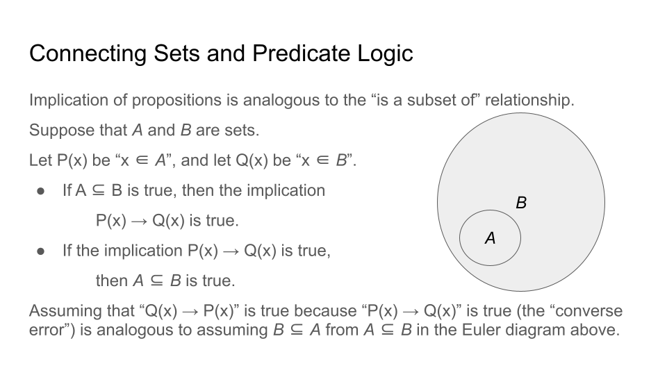
To see why the converse error is a fallacy, consider the following question: If you are told that \(c\) is an element of set \(B\) in the preceding image, can you determine whether \(c\) is an element of set \(A\)?
6.4. Proof Techniques
In this section several examples of formal mathematical proofs are given to illustrate different proof techniques. Many of the techniques correspond to certain rules of inference that were discussed earlier in this chapter.
Each proof starts by stating a conjecture, which is a proposition with undetermined truth value. The goal of each proof is to determine the truth value of the relevant conjecture.
To simplify the description of the proof techniques, we’ll only consider the case where the proof has a single premise \(p\), that is, we’ll always assume that our proof involves a single conditional \(p \rightarrow q\). This may seem like an oversimplification, but it is not: We are simply renaming the conjunction \((p_{1} \land p_{2} \land \ldots \land p_{n})\) of all of the actual premises by using the single propositional variable \(p\), that is we are defining \(p\) by the logical equivalence \(p \equiv (p_{1} \land p_{2} \land \ldots \land p_{n})\)
Here we’ll present examples of proofs using several different techniques. Most of these proofs establish an arithmetic fact that you probably have always known (or assumed) is True; instead, you can focus on the form of the proof: Note the steps that are used, and how the argument flows.
Another important proof technique, mathematical induction, will be discussed in a later chapter.
6.4.1. Direct Proof
In a direct proof, we make an argument that a conditional statement \(p \rightarrow q\) must be True. This means that we can assume that the premise \(p\) is True and apply modus ponens to prove that \(q\) must be True, too.
6.4.2. Proof By Contraposition
In a proof by contraposition, we make an argument that \(p \rightarrow q\) is True by instead first arguing that its contrapositive \(\neg q \rightarrow \neg p\) is True and secondly applying the logical equivalence of the conditional and its contrapositive. Start by assuming that the premise \(\neg q\) is True and apply modus ponens to prove that \(\neg p\) must be True, too, then apply logical equivalence.
6.4.3. Proof By Counterexample
In a proof by counterexample, we disprove a proposition of the form \((\forall x \in D) P(x)\) by arguing that there is at least one value \(c \in D\) such that \(\neg P(c)\) is True.
6.4.4. Proof by Contradiction
In a proof by contradiction, we disprove the proposition \(\neg p\) by making an argument that the conditional \(\neg p \rightarrow (q \land \neg q)\) must be True for some proposition \(q\) and apply the Contradiction Rule to conclude that \(p\) must be True.
Note: Sometimes, we argue instead that the proposition \(((\neg p \rightarrow q) \land (\neg p \rightarrow \neg q))\) must be True, and use the fact that this proposition is logically equivalent to \(\neg p \rightarrow (q \land \neg q)\) and apply the Contradiction Rule.
Here is another example of proof by contradiction.
6.4.5. Proof By Exhaustion (Proof By Cases)
Sometimes it is convenient to break a proof into a finite number of cases. For example, it may be easier to prove a statement that involves an integer by considering a first case where the integer is odd and a separate second case where the integer is even, then combining the two separate cases to create a single proof for all integers \(n.\)
In a general proof by cases, you make an argument that a conditional statement \((p_{1} \lor \cdots \lor p_{n}) \rightarrow r\) must be True. This means that if any one of the "cases" \(p_{i},\) where \(i \in \{ 1, 2, \ldots , n \},\) is True, you can apply the tautology \(p_{i} \rightarrow (p_{1} \lor \cdots \lor p_{n})\) and the transitivity rule of inference to prove that \(r\) must be True, too.
A proof by exhaustion is a special kind of proof by cases where the premise is of the form \((p_{1} \lor \cdots \lor p_{n} \lor \neg (p_{1} \lor \cdots \lor p_{n}) ).\) Notice that this premise must be True since if all of \(p_{1},\) \(p_{2},\)… \(p_{n}\) are False then \(\neg (p_{1} \lor \cdots \lor p_{n})\) is True.
If there are two cases, proof by exhaustion corresponds to using the "proof by cases" rule of inference discussed above in the section "Other Common Rules Of Inference." The tautology can be rewritten in the simpler form \(((p \rightarrow r) \land (\neg p \rightarrow r)) \rightarrow r\) because \(p \lor \neg p\) must always be True.
If there are more than two cases, this corresponds to using the tautology \(((p_{1} \rightarrow r) \land ... \land (p_{n} \rightarrow r) \land (\neg (p_{1} \lor \cdots \lor p_{n}) \rightarrow r)) \rightarrow r\).
7. Sequences and Recursion
CAUTION - CHAPTER UNDER CONSTRUCTION!
NOTICE: If you are NOT enrolled in the CSC 230 course that I teach at SFSU, you probably are looking for the “public version” of the book, which I only update between semesters. The version you are looking at now is the “CSC230 version” of the book, which I will be updating throughout the semester.
This chapter was last updated on October 12, 2025.
Edited definition of recursively-defined function.
Added material to the section about the Towers Of Hanoi.
Sequences are functions with domain a nonempty subset of the natural numbers. That is, sequences are ordered lists of objects indexed by some or all of the natural numbers. The indexed objects in the list are called the terms of the sequence and may be any kind of object - numbers, sets, functions, strings, steps of a proof, steps of an algorithm, etc.
Recursion is a process that you can use to define an object, compute a value, or describe the construction of an object or set of objects, by using a sequence of steps where each step after the initial step refers to one or more previously completed steps.
Key terms and concepts covered in this chapter:
-
Sequences
-
Recursive mathematical definitions
-
Recursive definitions of sequences and functions
-
Factorials
-
Arithmetic and geometric progressions
-
The Fibonacci sequence (also called the Fibonacci numbers)
-
Other sequences and functions
-
-
Recursive definitions of sets of objects (e.g., rooted trees, valid Java identifiers)
-
The "Towers of Hanoi" game
-
-
Recurrence relations
-
Solving recurrence relations
-
7.1. Sequences
A sequence is a function \(s\) from a nonempty subset of the natural numbers \(\mathbb{N} = \{ 0, 1, 2, 3 \ldots \}\) to a set \(C.\) That is, the domain of the sequence is some set of nonnegative integers, and the codomain can be any set. Each "input" value of \(n\) in the domain is called an index. The "outputs" of the sequence are called the terms of the sequence, and are usually denoted by \(s_{n},\) which is usually used instead of the function notation \(s(n),\) but the meaning is the same: The output value that corresponds to the input \(n.\)
7.1.1. Sequences of Numbers
Two common ways to describe or define a sequence of numbers are
-
a single formula, called a closed form for the sequence, that can be used to compute a term from the value of the index \(n,\) or
-
a recursive rule that includes
-
stating the values of the first few terms of the sequence, called the initial value(s) of the sequence, and
-
a recurrence relation that describes how the \(n\)th term of the sequence \(a_{n}\) can be computed using one or more terms that have index less than \(n.\)
-
In this subsection, several examples of sequences of numbers are presented. You may have seen some of these sequences in your previous mathematics experience but others may be new to you.
An arithmetic sequence is a sequence of numbers generated by a linear expression.
A geometric sequence is a sequence of numbers generated by an exponential expression.
The factorial is usually defined using a recurrence relation, but with its own notation that does not use a subscript for the index.
The next sequence is the very famous Fibonacci numbers, named for the Italian mathematician Fibonacci who was also known as Leonardo of Pisa. However, this sequence and its properties were known and discussed by Indian poets and mathematicians such as
Pingala,
Virahanka,
and
Hemachandra
before Fibonacci was born. The sequence became known to Europeans when Fibonacci used the sequence in his 1202 book Liber Abaci to solve a counting problem that involves breeding pairs of rabbits
The book Liber Abaci ("Book of Calculation") is credited with popularizing the use of the base-ten Hindu-Arabic numeral system in Europe, too.
7.1.2. Non-numerical Sequences
As mentioned above, the terms of a sequence can be any object. Here are some examples.
The ordered list of steps used in an algorithm is a sequence.
7.2. Recursion
A recursive definition of a class of objects consists of two steps.
| Basis Step |
Specify the foundational (usually, the simplest) objects in the class of objects. |
| Recursion |
Describe how to build new objects from one or more already-constructed objects in the class of objects. |
7.2.1. Recursively-Defined Structures
For some mathematical objects, it is easier to describe the construction of the objects using a recursive definition.
You may recall that well-formed formulae were defined in the Logic chapter using a recursive definition. We formalize that definition here.
In the next example, we describe how to construct rooted trees, a type of graph.
A rooted tree is a type of graph. Graphs are described informally in the Introducing Discrete Mathematics chapter.
The set of rooted trees, is defined recursively as follows.
| Basis Step |
A single vertex r is a rooted tree. The vertex r is called the root node of this rooted tree. |
| Recursion |
You can construct a new rooted tree from already-constructed rooted trees as follows. Suppose you have a nonempty finite set of “old” rooted trees (that is, already-constructed rooted trees) such that |
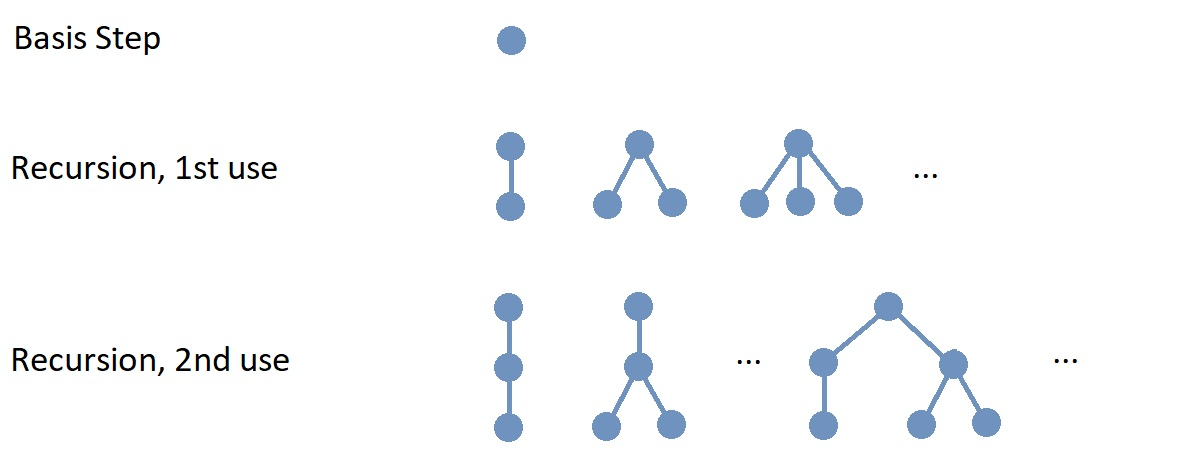
The preceding image shows the basis step and represents, in part, the results of the first and second uses of the recursion step. In the image, the new root nodes created at each recursion step appear at the top of the newly-created rooted trees. In each rooted tree, edges are treated as if they are directed “down,” away from the new root node; this will be discussed in more detail in the Trees chapter.
Notice that infinitely-many rooted trees are constructed at each use of the recursion step, so we cannot show all the rooted trees produced at any step other than the basis step. Also, we would need to complete infinitely many steps to construct all possible rooted trees, but any one particular rooted tree you want to construct will be produced after only finitely many uses of the recursion step.
7.2.2. Recursively-Defined Functions
A recursively defined function has two parts:
-
Basis Step: Specify the value of the function at one or more small input values.
-
Recursion Step: Give a rule for computing the function’s output value at an integer based on the output values at one or more smaller integers.
A recursive definition of a function is similar to a recurrence relation, but uses function notation.
7.3. Solving Recurrence Relations
Recall from earlier in this chapter that a recurrence relation is used to recursively define a sequence of numbers, based on one or more initial conditions, that is, the value(s) of the lowest-indexed term(s).
The phrase "solving a recurrence relation" means finding a closed form that defines the same sequence as the recurrence relation.
There are techniques used to solve certain classes of recurrence relations. For now, we will focus on only one case, the class of second-order linear homogeneous recurrence relations.
7.4. Towers Of Hanoi
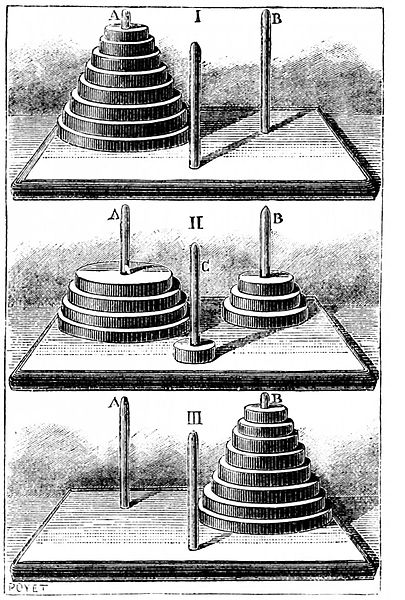
The Towers of Hanoi is a game that was introduced and sold by the French mathematician Édouard Lucas in the 1880s. Lucas stated that the game is "professedly of Indo-Chinese origin" but it seems that Lucas invented this story to market the game.
Image credit: "PSM V26 D464 The tower of hanoi.jpg". This work is in the public domain in its country of origin and other countries and areas where the copyright term is the author’s life plus 70 years or fewer.
At the start of the game, a set of disks of different radii are stacked on a single peg to form a "tower." The disks are stacked so that the radii of the disks decrease as you move up the stack. There are also two empty pegs. The game is won by moving the stack of disks from the original peg to another peg using the following rules
-
Only one disk can be moved at a time.
-
The disk at the top of a stack can be moved to the top of another stack or on to an empty peg.
-
A disk can never be placed on top of a disk that has a smaller radius.
The Towers of Hanoi can be used to explore recursive algorithms, complexity of algorithms, and recurrence relations, based on the following questions.
-
What is the minimal number of moves needed to win the game when there is 1 disk? 2 disks? 3 disks? \(n\) disks?
-
What relationship (if any) is there between the minimal number of moves needed to win an \(n\)-disk game and the minimal number of moves needed to win an \((n-1)\)-disk game?
MORE TO COME!
8. Functions
CAUTION - CHAPTER UNDER CONSTRUCTION!
NOTICE: If you are NOT enrolled in the CSC 230 course that I teach at SFSU, you probably are looking for the “public version” of the book, which I only update between semesters. The version you are looking at now is the “CSC230 version” of the book, which I will be updating throughout the semester.
This chapter was last updated on March 11, 2025.
Contents locked until 11:59 p.m. Pacific Standard Time on May 23, 2025.
Informally, a function \(f\) from set D to set C is a rule that assigns to each input element in D exactly one output element from C. The set D is called the domain of the function, and the set C is called the codomain of the function. This informal definition was given in the chapter Introducing Discrete Mathematics.
The informal definition implies that every element in the domain D is an "input" that is assigned an output value in the codomain C. The informal definition does not imply that every element in the codomain C is an output for some input in the domain D. The highlighted sentence may seem unimportant since you usually only care about the outputs you can actually get from a function, but the example presented in the next section shows why it is important to be precise about what set the codomain is. A formal definition of function is introduced in this chapter to address this need for precision.
Key terms and concepts covered in this chapter:
-
Functions
-
Domain
-
Codomain
-
Range
-
-
Properties of functions (injectivity, surjectivity, bijectivity)
-
A bijective function is the same as a one-to-one correspondence
-
An injective function is one that assigns every pair of different inputs to a pair of different outputs
-
A surjective function is one whose range is equal to its codomain (that is, every element of the codomain is an output assigned to one or more inputs)
-
A bijective function is both injective and surjective
-
-
Inverse functions
-
Composition of functions
8.1. Why Specifying the Codomain is Important
The following example compares two implementations, in different programming languages, of the "same" function: The input values are the same, and the rule that assigns to each input its one and only output is the same. However, the two implementations use different codomains which effects how the output values can be used.
The formal definition given in the next section will let us distinguish between two functions that use the same rule and have the same domain but have different codomains.
8.2. A Formal Definition Of Function
Why would we need such a highly technical formal definition? The reason why the ordered triple is used in the definition is that we need to be able to distinguish two functions that have the same graph, as a set of ordered pairs, but different codomains. Two functions can have different codomains even if their graphs, as sets of ordered pairs, are the same set (Notice that if two functions have the same graph then they must have the same domain.) If this is not clear, see the example "Three closely-related functions, no two of which are equal," which comes after the definitions listed below.
-
We write \(f : A \rightarrow B\) to state that \(f\) is a function from set \(A\) to set \(B.\)
-
We often refer to the ordered triple as "f" without explicitly mentioning the other two members of the ordered triple. That is, we refer to the function as its set of ordered pairs \(f\), but it is very important to remember that the actual definition includes the domain and codomain, too.
-
It is important to note that the graph of \(f\) is the set of ordered pairs which we often represent by plotting points, but that plot is only a representation of the graph (in the same way that "five" and "cinco" are verbal representations of a number but are not the number itself.)
-
We write \(f(a)=b\) instead of \((a,\, b) \in f\). The value \(b = f(a)\) is called the image of \(a\) assigned by \(f,\) and \(a\) is called the pre-image of \(b.\)
-
The range of \(f\) is the set \(\{ f(a) : a \in A \}\), that is, the set of all images (output values) assigned by \(f.\) The range is the set of \(b \in B\) such that there is at least one ordered pair \(( a, \, b) \in f.\)
-
Two functions are equal if they have the same graph, the same domain, and the same codomain. That is, the functions \((f,\, A,\, B)\) and \((g,\, S,\, T)\) are equal if they are identical as ordered triples: \(f = g\) and \(A = S\) and \(B = T.\) We can also simply say that "\(f\) and \(g\) are the same function."
-
Notice that the graph \(f\) in the formal definition replaces the rule used in the informal definition. Given the graph, which is the set of ordered pairs, we can state a rule as "given an input \(a \in A,\) the output is the one \(b \in B\) such that \((a,\, b) \in f.\)" This is exactly how you would use a table of values to represent a function: Find the row with the input value then choose the value in the output column
|
The graph (i.e., the set of ordered pairs), the domain, and the codomain determine the function, NOT the formula, words, table, plot, or code used to describe a rule for the function.
The graph of a function determines how to assign each input to its output. For example, the functions \(f: \mathbb{R} \rightarrow \mathbb{R}\) and \(g: \mathbb{R} \rightarrow \mathbb{R}\) defined by the formulae \(f(x) = |x|\) and \(g(x) = \sqrt(x^{2})\) are equal, and in fact are one and the same function, because \(f = g\) as sets, so the "two" functions have the same graph, the same domain, and the same codomain. The "two" functions are just two ways of describing the same ordered triple. |
8.3. Properties of Functions
In this subsection you will learn about several properties of functions.
8.3.1. Injective Functions
A function \(f : A \rightarrow B\) is injective if distinct elements of the domain \(A\) are mapped to distinct elements of the range.
That is, for all \(a_1\) and \(a_2\) in \(A,\) if \(a_1 \neq a_2\) then \(f(a_1) \neq f(a_2).\)
Using the contrapositive, this can be stated as: For all \(a_1\) and \(a_2\) in \(A,\) if \(f(a_1) = f(a_2)\) then \(a_1 = a_2.\)
Note: Injective functions are also called one to one functions. The Remix avoids this term because it is easy to confuse "one to one function" with "one-to-one correspondence."
8.3.2. Surjective Functions
A function \(f\) from the set \(A\) to the set \(B\) is surjective if the image set of \(A\) is the entire set \(B\). This means than for each element \(b\) in the codomain \(B,\) there is some element \(a \in A\) with \(f(a)=b\).
Note: Surjective functions are also called onto functions.
Consider the functions
\(f : \mathbb{Z} \rightarrow \mathbb{Q}\) defined by \(f(n) = 2^{n}\)
\(g : \mathbb{Z} \rightarrow \mathbb{Z}\) defined by \(g(n) = n^{2},\) and
\(h : \mathbb{Z} \rightarrow \mathbb{Z}\) defined by \(h(n) = n + 2,\) and
\(k : \mathbb{Z} \rightarrow \mathbb{Z}\) defined by \(k(n) = \frac{1}{4}((-1)^n (2n+1) - 1).\)
\(f\) is not surjective since it is not possible for \(2^{n}\) to have a value that is less than or equal to 0.
\(g\) is not surjective because is not possible for \(n^{2}\) to have a value that is less than 0.
\(h\) is surjective because every \(b\) in the codomain \(\mathbb{Z}\) is an output for some input: Notice that \(h(b-2) = (b-2+2) = 2.\)
\(k\) is surjective because every \(b\) in the codomain \(\mathbb{Z}\) is an output for some nonnegative input - for inputs \(n \geq 0,\) the outputs \(k(n)\) are shown in the lower row of the image.
Notice that whether a function is surjective depends on what the function’s codomain. This is, again, why the formal definition of function is needed.
8.3.3. Bijective Functions
A function \(f\) is bijective if it is both injective and surjective.
8.4. Inverse Functions
Informally, a function \(f\) is invertible if each \(b\) in the codomain \(B\) is assigned to exactly one input \(a\) in the domain \(A.\)
Formally, a function \(f : A \rightarrow B\) is invertible if the ordered triple \((\{(b, a) \, | \, (a, b) \in f \},\, B,\, A)\) is a function.
The set \(\{(b, a) \, | \, (a, b) \in f \}\) is usually denoted by \(f^{-1}\) even in cases when \(f\) is not invertible.
For example if \((a,b)\), corresponds to \(f(a)=b\) , then \( f^{-1}: B \rightarrow A\), corresponds to \( f^{-1}(b)=a\).
The following theorem shows that invertibility of a function is equivalent to bijectivity, or a function being both injective and surjective.
|
Being able to solve an equation, amounts to being able to invert a function. Notationally, solving \(f(x) =b\) means solving for \(x\). Using inverses \(f(x) =b\) is solved \(x=f^{-1}\left(b\right)\). |
Consider, for example, \(f\left(x\right)=x^3\) we know
Solving \(f\left(x\right)=2\) means solving \(x^3=2\). To solve \(f\left(x\right)=2\), we use \(x=f^{-1}\left(8\right)\), which in this case means,
An easy check \( f\left(2\right)=2^3=8\) and
Functions can, in many cases, be visualized graphically. For example when mapping from the real line \(\mathbb{R}\) to the real line such maps are viewed on a Cartesian plane.
In Appendix: Library of Functions, several functions and their plots are shown to illustrate the important concepts of functions, including domain, codomain, range, and invertibility.
8.5. The Algebra of Functions
If two functions \(f\left(x\right)\) and \(g\left(x\right)\) have the same domain \(A\) and same codomain \(\mathbb{R},\) then you can combine these functions using the operations addition, subtraction, multiplication, and division.
8.6. Composition of Functions
Suppose \(g:A\rightarrow B\) and \(f:B\rightarrow C\), then the functions \( f\) and \(g\), can be composed to obtain a function \(h:A\rightarrow C\), denoted as follows,
\(h\left(x\right)=\left(f\circ g\right)\left(x\right)=f\left(g\left(x\right)\right)\) provided \(x\ \in\ A\) and \(g\left(x\right)\in B\).
Notice, in the last example, that \(g\left(x\right)\) undoes \(f\left(x\right)\), in the following sense:
\(f:1\rightarrow 2\) and \(g:2\rightarrow 1\), or the ordered pair \(\left(1,2\right)\) in \(f\), corresponds to \(\left(2,1\right)\) for \(g\).
\(f:2\rightarrow 9\) and \(g:9\rightarrow 2\), or the ordered pair \(\left(2,9\right)\), in \(f\), corresponds to \(\left(9,2\right)\) for \(g\).
\(f:3\rightarrow 28\) and \(g:28\rightarrow 3\), or the ordered pair \(\left(3,28\right)\), in \(f\), corresponds to \(\left(28,3\right)\) for \(g\).
\(f:x\rightarrow x^3+1\) and \(g:x^3+1\rightarrow x\), or the ordered pair \(\left(x,x^3+1\right)\), in \(f\), corresponds to \(\left(x^3+1,x\right)\) for \(g\).
The function \$ g(x))= root(3)(x-1) \$ is said to be the inverse of the function \(f\left(x\right)=x^3+1\). We have shown explicitly that \(\left(g\circ f\right)\left(x\right)=x\).
8.6.1. Inverse Functions and Composition
Notice that if you happen to have two functions \(f : A \rightarrow B\) and \(g : B \rightarrow A\) such that \((g \circ f)(a) = g(f(a)) = a\) for every \(a \in A\) and \((f \circ g)(b) = f(g(b)) = b\) for every \(b \in B,\) then \(f\) and \(g\) are inverse functions.
8.7. Exercises
Remixer’s Note: This section is taken from the original “Discrete Math” book with only minor changes.
-
What can be said about the relation \(f:A\rightarrow B\), if
-
\(\exists z\in B\forall x\in A,f\left(x\right)\neq z\)
-
\(\exists x,y \in A, \exists z\in B,\left(x\neq y\right)\bigwedge\left(f\left(x\right)=f\left(y\right)=z\right)\)
-
\(\forall x,y\in A, \left(f\left(x\right)=f\left(y\right)\right)\ \rightarrow\left(x=y\right)\)
-
\(\forall x,y\in A,\left(x\neq y\right)\rightarrow\left(f\left(x\right)\neq f\left(y\right)\right)\)
-
\(\forall z\in B, \exists x,f\left(x\right)=z\)
-
\(\exists x,y\in A,\left(f\left(x\right)=f\left(y\right)\right)\bigwedge\left(x\ \neq\ y\right)\)
-
-
Explain why exponential function \(f(x)=2^x\) is not surjective from \(f: \mathbb{R} \rightarrow \mathbb{R}\), but is in fact a bijection from \(f: \mathbb{R} \rightarrow \mathbb{R}^+\).
-
Use properties of logarithms to show that \(f\left(x\right)=2^x\) and \(g\left(x\right)=\log_2{x}\), where \(f, g: \mathbb{R} \rightarrow \mathbb{R}\), are inverses by verifying that \(f\left(g\left(x\right)\right)=g\left(f\left(x\right)\right)=x\).
-
Use properties of logarithms to show that \(f\left(x\right)=10^x\) and \(g\left(x\right)=\log{x}\), where \(f, g: \mathbb{R} \rightarrow \mathbb{R}\), are inverses by verifying that \(f\left(g\left(x\right)\right)=g\left(f\left(x\right)\right)=x\).
-
Show that the function \(f\left(x\right)=5x-3\), from \(f: \mathbb{R} \rightarrow \mathbb{R}\), is bijective and find its inverse.
-
Show that the function \(f\left(x\right)=2x^3-1\), from \(f: \mathbb{R} \rightarrow \mathbb{R}\) is bijective and find its inverse.
-
Consider the function \(f(x) = \left \lceil x \right \rceil\) where \(f:\mathbb{R}\rightarrow\mathbb{Z}\).
-
Is the function a surjection? Explain.
-
Is the function an injection? Explain
-
Is the function a bijection? Explain
-
Is the inverse mapping a function? Why or why not?
-
Evaluate
-
\(f\left(-2.1\right)\)
-
\(f\left(-1.9\right)\)
-
\(f\left(1.5\right)\)
-
\(f\left(1.9\right)\)
-
\(f\left(2\right)\)
-
\(f\left(2.3\right) \)
-
-
Suppose \(g\left(x\right)=2x\), with \(f\left(x\right)=\left\lceil x\right\rceil\). Evaluate the following:
-
\(f\left(g\left(2.3\right)\right)\)
-
\(g\left(f\left(2.3\right)\right)\)
-
-
-
Explain why ceiling function \( \left \lceil x \right \rceil\) is not surjective from \(f: \mathbb{R} \rightarrow \mathbb{R}.\)
-
Consider the function \(f(x) = \left \lfloor x \right \rfloor\) where \(f:\mathbb{R}\rightarrow\mathbb{Z}\).
-
Is the function a surjection? Explain.
-
Is the function an injection? Explain
-
Is the function a bijection? Explain
-
Is the inverse mapping a function? Why or why not?
-
Evaluate
-
\(f\left(-5.1\right) \)
-
\(f\left(-3.9\right)\)
-
\(f\left(-3.2\right)\)
-
\(f\left(5\right) \)_
-
\(f\left(5.3\right)\)
-
-
Suppose \(g\left(x\right)=3x\), with \(f\left(x\right)=\left\lfloor x\right\rfloor\). Evaluate the following:
-
\(f\left(g\left(5.3\right)\right)\)
-
\(g\left(f\left(5.3\right)\right)\)
-
-
-
The absolute value function, denoted \(f(x)=|x|\), where \(f\left(x\right):\mathbb{R} \rightarrow \mathbb{R}\), gives the distance from \(x\) to \(0\). For example, \(f\left(2.5\right)=\left|2.5\right|=2.5\). And \(f\left(-4.5\right)=\left|-4.5\right|=4.5\). Notice that if \(x \geq 0\), then \(\left|x\right|=x\). However if \(x<0\), then \(\left|x\right|=\ -x\). We can state this using the notation for piecewise functions:
\$f(x) = |x|={( x, if x ≥ 0),(-x,if x < 0):}\$-
Graph \(f\left(x\right)=|x|\), for -\(10\ \le x\ \le10\)
-
Evaluate
-
\(f(-5)=|-5|\),
-
\(f(-2.5)=|-2.5|\),
-
\(f(3.5)=|3.5|\).
-
-
Show that \(f\left(x\right)=\left|x\right|\), with \(f:\mathbb{R}\rightarrow \mathbb{R}\), is not injective.
-
Show that \(f\left(x\right)=\left|x\right|\), with \(f:\mathbb{R}\rightarrow \mathbb{R}\), is not surjective.
-
Consider \(g\left(x\right)=3x+2\), with \(g:\mathbb{R}\rightarrow \mathbb{R}\), and \(f\left(x\right)=|x|\). Find and simplify the following:
-
\(\left(g\circ f\right)\left(x\right)\)
-
\(\left(f\circ g\right)\left(x\right)\)
-
-
-
A real-valued function, \(f: \mathbb{R} \rightarrow \mathbb{R}\), is said to be strictly increasing if whenever \$x<y\$, then \$f(x)<f(y)\$.
-
State this using logical quantifiers.
-
State a similar definition for a strictly decreasing function, and then translate using logical quantifiers.
-
9. Relations
CAUTION - CHAPTER UNDER CONSTRUCTION!
NOTICE: If you are NOT enrolled in the CSC 230 course that I teach at SFSU, you probably are looking for the “public version” of the book, which I only update between semesters. The version you are looking at now is the “CSC230 version” of the book, which I will be updating throughout the semester.
This chapter was last updated on October 20, 2025.
Revised the sections/subsections on partial orders, well-ordering, and modular arithmetic.
Made other minor revisions and fixed typos.
Relations are used to describe an association of data.
For example, imagine a university database of students. The database needs to have a record for each student, and the student’s record needs to include fields for the student’s name(s), the unique student ID number for the student, the student’s current status, a list of courses that the student has enrolled in or has completed (along with the grade earned in each completed course,) and possibly other data associated with the student. One way to visualize the database is as a two-dimensional table, similar to a spreadsheet worksheet, where each row corresponds to a record and each column corresponds to a field; each row can be treated as an ordered \(n\)-tuple, where \(n\) is the number of fields.
In this chapter, you will learn about the formal definition of relation, operations and properties of relations. You will also learn about some special types of relations, namely partial orderings and equivalence relations. As a special case of equivalence relations, you will learn about congruence relations of integers as well as modular arithmetic.
Key terms and concepts covered in this chapter:
-
Relations
-
Properties of relations (reflexivity, symmetry, transitivity, and other properties)
-
Equivalence relations
-
Equivalence classes
-
-
Modular arithmetic
-
Congruences
-
-
Partial orders
-
Well orderings
9.1. Definition of Relation
Informally, a relation on two or more sets is an association between elements of those sets.
Formally, a relation is a subset of a Cartesian product of two or more sets.
For simplicity, it is assumed in this textbook that the number of sets used to form the Cartesian product is finite. It is possible to define relations as subsets of a Cartesian product of infinitely many sets, in which case the elements of the relation are infinite sequences.
Here are several examples of relations.
Notice that for any sets \(A_{1}, \, A_{2}, \, \ldots \, A_{n},\) where \(n \geq 2\) is a natural number, we always have the following two relations:
-
\(\emptyset,\) called the empty relation. This relation is also called the void relation and trivial relation in other sources.
-
\(A_{1} \times A_{2} \times \cdots \times A_{n},\) called the universal relation.
9.2. Binary Relations on a Single Set
In many cases, the two domains of a binary relation are the same set; for example, the relation may involve comparing two elements of a set S in some way. In this case, the domain \(S\) is mentioned only once: A binary relation on set S is any subset \(R\) of the cartesian product \(S \times S\), that is, \(R \subseteq S \times S.\)
In the case of a binary relation on \(S,\) we often write \(aRb\) to mean the same thing as \((a,b) \in R.\) This notation may make more sense after reading the following example.
9.2.1. Operations on Binary Relations on a Set
Given binary relations \(Q\) and \(R\) on a set \(S,\) we can define several other relations in terms of \(Q\) and \(R.\) These operations are likely familiar to you as operations on functions but they also work for binary relations on a single set.
-
The inverse of \(R\) is the relation \(R^{-1} = \{ (b,a) \, | \, (a,b) \in R \}.\)
-
The composition of Q and R is \(R \circ Q = \{ (a,c) \, | \, (a,b) \in Q \land (b,c) \in R \}.\)
-
The n th power of \(R\) is defined recursively for all \(n \in \mathbb{N}\) as follows.
-
\(R^{0} = \mathbf{id}_S\)
-
\(R^{k+1} = R \circ R^{k}\) for natural numbers \(k > 0.\)
The recursion step uses \(k\) instead of \(n\) in preparation for the type of arguments used in the chapter on proof by mathematical induction.
-
Building on the \(n\)th powers of \(R,\) we can define two relations.
-
\(R^{+}\) is the relation \(\{ (a,b) \in S \times S \, | \, (a,b) \in R^{k} \text{ for some positive integer } k \}.\) That is, \(R^{+}\) is the union of all the positive \(n\)th powers of \(R.\)
-
\(R^{*}\) is the relation \(\{ (a,b) \in S \times S \, | \, (a,b) \in R^{k} \text{ for some natural number } k \}.\) That is, \(R^{*}\) is the union of all the natural number \(n\)th powers of \(R.\)
Notice that \(R^{*} = \mathbf{id}_S \cup R^{+}.\)
9.2.2. Properties of Binary Relations on a Set
In this subsection we define five properties that a relation may satisfy.
The following theorem can make it easier to determine when a relationship has each of the five properties. The proof of the theorem is an exercise.
9.2.3. Closures of Binary Relations with Respect to a Property
For each of the properties reflexivity, symmetry, and transitivity, we define the closure with respect to the property of a relation \(R\) as follows: The closure is the smallest relation that has the property and includes all the elements of \(R.\) That is, you start with \(R\) and try to insert in just enough ordered pairs, if any are needed, to make sure that the new relation has the desired property.
The following theorem justifies that the reflexive closure, symmetric closure, and transitive closure exist for any relation \(R.\) The proof of the theorem is an exercise.
Notice that we can also define the reflexive and transitive closure of a relation \(R\) as the relation \(R^{*},\) which is the reflexive closure of the transitive closure of \(R.\)
However, for some properties, the closure of a relation \(R\) with respect to the property may not exist!
9.3. Equivalence Relations
A binary relation \(R\) on a set \(S\) is called an equivalence relation on \(S\) if \(R\) is reflexive, symmetric, and transitive.
A first example of an equivalence relation is the diagonal, that is, the equality relation. Another example is given below.
Given an equivalence relation \(R\) on the set \(S\) and an element \(x \in S,\) we define the equivalence class of \(x\) to be \([ x ]_{R} = \{ y \in S \, | \, (x,y) \in R \}.\)
9.4. Order Relations on a Set
It is often useful to be able to compare elements of a set, based on some key property. In this subsection, several examples of such order relations will be discussed.
9.4.1. Partial Orderings
A binary relation \(R\) on a set \(S\) is called a partial order on \(S\) if \(R\) is reflexive, antisymmetric, and transitive.
For any set \(S,\) each of the relations \(\subseteq\) and \(\subset\) is a partial order on \(\mathcal{P}(S),\) the power set of \(S.\)
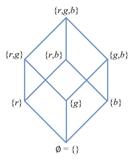
As an example, for the set \(S = \{ r, g, b \},\) the image shows a Hasse diagram that represents the \(\subset\) relation on the power set \(\mathcal{P}(S).\) Notice that each line segment in the Hasse diagram connects a first subset of \(S\) to a second subset of \(S\) that is “immediately above” the first subset in the following sense: Each member of the first subset is also a member of the second subset, but the second subset has one additional member. In the Hasse diagram, two different subsets \(A\) and \(B\) satisfy \(A \subset B\) if and only if there is a “path up” from \(A\) to \(B\) that uses one or more of the line segments.
Total Orderings
A total ordering of a set \(S\) is a partial order \(R\) on \(S\) that has the additional property \((\forall x \in S)(\forall y \in S)(xRy \lor yRx).\)
Well-Orderings
A well-ordering of a set \(S\) is a total ordering \(R\) on \(S\) that has the additional property that every nonempty subset of \(S\) contains a least element with respect to the order relation.
One of the most important examples of a well-ordering in mathematics is the relation \(\leq\) on the set of natural numbers \(\mathbb{N}.\)
In the Remix, the Well-Ordering Principle is treated as an axiom, a statement that is assumed to be True about the set of natural numbers.
The Well-Ordering Principle may seem like an “obviously True” statement. To understand why mathematicians would make it clear that they are assuming that this principle is True is to understand what “infinity” means.
-
First, suppose that you are told that the subset \(A\) of \(\mathbb{N}\) contains the element 10. You can use a brute‑force method to determine the least element of \(A:\) Just ask the following sequence of 10 questions, in the order shown. \[ \text{“Is 0 in \(A?,\)” “Is 1 in \(A?,\)” \(\ldots\), “Is 9 in \(A?\)”} \] If the answer is “No” to all 10 of these questions, then 10 itself is the least element in \(A\), otherwise, the least number in \(A\) is the first value of \(k\) for which the answer to the question “Is \(k\) in \(A?\)” is “Yes.”
-
Next, suppose that you are given a new set \(S\) and told that the number \(10^{10^{10^{10^{10}}}}\) is in \(S.\) You again could try to use the brute‑force method of asking the sequence of \(10^{10^{10^{10^{10}}}}\) questions: \[ \text{“Is 0 in \(S?,\)” “Is 1 in \(S?,\)” \(\ldots\), “Is \(\left( 10^{10^{10^{10^{10}}}}-1 \right)\) in \(S?\)”} \] but even if it took only 1 nanosecond to ask and answer each question, the integer \(10^{10^{10^{10^{10}}}}\) is greater than the number of nanoseconds estimated for our universe to reach its final energy state! That is, it is possible that the answer to one of these questions is “Yes” but that you would never be able to ask that question before the universe ends! Notice that you can use formal logic to justify that either the answers to all of those questions would be “No” or that at least one of the questions would have the answer “Yes” — asking the sequence of questions would determine the least element in \(S\) if you had time to ask enough of the questions, but you (and humanity itself) may not have that much time. For this reason, mathematicians assume that the least element of the set \(S\) exists.
Notice that a “timeless being” could know all the answers.
9.5. Modular Arithmetic (Revision in Progress!)
Let \(m\) stand for some positive integer constant that is greater than 1. The relation congruence modulo \(m\) is defined to be \[\{ (a, b) \in \mathbb{Z} \times \mathbb{Z} \, : \, m \text{ divides } (a-b) \}.\] The symbol \(\equiv_{m}\) is used to represent congruence modulo \(m\), so \[a \equiv_{m} b \text{ if and only if } m \text{ divides } (a-b).\]
As an example, \(13 \equiv_{3} 7\) because \(3\) divides \(13-7.\) Another way to see that \(13 \equiv_{3} 7\) is to notice that both \(13\) and \(7\) leave a remainder of \(1\) when divided by \(3\) using integer long division.
Notice that the relation \(\equiv_{2}\) is the same as the parity relation discussed in an example earlier in this chapter. As discussed in that example, \(\equiv_{2}\) is an equivalence relation. In fact, for each positive integer constant \(m\) that is greater than 1, the relation \(\equiv_{m}\) is an equivalence relation.
We can also do “arithmetic” directly with the equivalence classes of the \(\equiv_{m}\) relation. The following example may make this more clear.
You likely learned, when you were quite young, that some integers are called "even" and other integers are called "odd."
Notice that every integer is either even or odd but not both, which means that the set \[\{ \text{the set of all even integers}, \, \text{the set of all odd integers} \}\] or more formally \[\{ \{ \ldots, -4, -2, 0, 2, 4, \ldots \}, \, \{ \ldots, -3, -1, 1, 3, \ldots \} \}\]forms a partition of the set \(\mathbb{Z}\) of integers. This partition corresponds to the relation \(\equiv_{2},\) that is, congruence modulo 2. The set of all even numbers is the equivalence class \([ 0 ]_{\equiv_{2}}\) and the set of all odd numbers is the equivalence class \([ 1 ]_{\equiv_{2}}.\)
You may have learned how to do arithmetic with "Even" and "Odd," too, as shown in the tables.
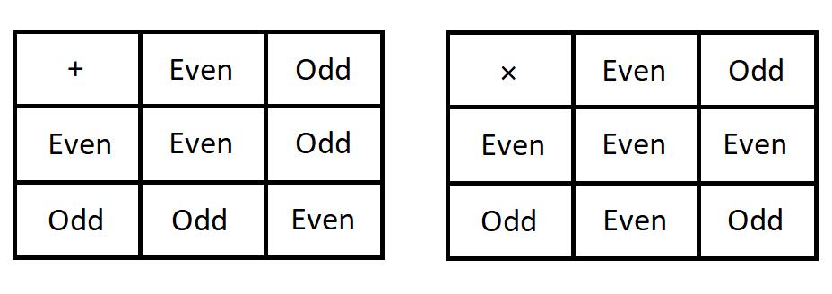
When you did arithmetic with "Even" and "Odd," you were really doing arithmetic with the equivalence classes \([ 0 ]_{\equiv_{2}}\) and \([ 1 ]_{\equiv_{2}}.\) For example, it will not matter which two odd numbers you add, the result must be even because the two numbers were odd. You can just do the operations on the remainders that you get after dividing by 2, which corresponds to adding the equivalence classes: \([ 1 ]_{\equiv_{2}} + [ 1 ]_{\equiv_{2}} = [ 1+1 ]_{\equiv_{2}} = [ 2 ]_{\equiv_{2}} = [ 0 ]_{\equiv_{2}}\) where the last equality is True because \(2\) and \(0\) belong to the same equivalence class (that is, they are both even numbers.)
The following theorem proves that you can do addition and multiplication with the remainders (or, what amounts to the same thing, the equivalence classes) in the same way as was done with Evens and Odds in the previous example for the relation \(\equiv_{m},\) where \(m\) can be any integer greater than 1.
For example, we can write \(9 + 5 \equiv_{12} 2\) (This is an example of "clock arithmetic" using a 12-hour clock: 5 hours after 9 o’clock will be 2 o’clock.)
MORE TO COME!
10. Counting: Permutations and Combinations
CAUTION - CHAPTER UNDER CONSTRUCTION!
NOTICE: If you are NOT enrolled in the CSC 230 course that I teach at SFSU, you probably are looking for the “public version” of the book, which I only update between semesters. The version you are looking at now is the “CSC230 version” of the book, which I will be updating throughout the semester.
This chapter was last updated on March 17, 2025.
Contents locked until 11:59 p.m. Pacific Standard Time on May 23, 2025.
Many problems can be solved by counting the number of possible outcomes when choosing \(r\) elements from a set that contains \(n\) elements, with no repetition allowed (that is, each element can only be counted once). To be clear, this assumes that \(r\) and \(n\) are natural numbers and \(r \leq n.\)
Some of these problems involve choosing an ordered sequence of \(r\) elements while other problems involve choosing a subset of \(r\) elements.
This chapter presents techniques for doing this type of counting. These techniques are built on the ones you studied in the Counting: Arithmetic Techniques chapter.
Key terms and concepts covered in this chapter:
-
Permutations and combinations
-
Basic definitions
-
Pascal’s identity
-
The binomial theorem
-
-
binomials
10.1. The Factorial Of A Number
The factorial is a function defined for all natural numbers as described below.
10.2. Permutations
A permutation of a set of elements is an ordered arrangement of the elements without repetition of elements. A permutation may involve every element of the set, or only some of the elements of the set. That is, a permutation is a sequence of elements from the set, where no element can appear more than once in the sequence.
Note: If you studied outside the USA, you may have learned that a permutation must involve every element of the set, and that the term variation is used when the arrangment involves only some (but not all) of the elements of the set. In this textbook, all of these are called permutations.
Consider the last four uppercase English letters \(W, X, Y, Z\).
-
\(WXYZ, XWYZ, WXZY\) are permutations of the letters taken four at a time
-
\(XZW, WXY, WXZ\) are permutations of the letters taken three at a time
-
\(WX, WY, ZX\) are permutations of the letters taken two at a time
Note: To be more formal, the sequences above could be written as tuples of the form \((W, X, Y, Z),\) \((X, W, Y, Z),\) \((W, X, Z, Y),\) and so on, but the notation used is simpler without the extra symbolic clutter of parentheses and commas.
Notice that no letter is repeated in a permutation.
How can you count all the possible permutations of a set? For small sets like the set of the last four uppercase English letters, you could list all the possible permutations of \(W, X, Y, Z\) to determine that there are 24 permutations of the letters taken four at a time, 24 permutations of the letters taken three at a time, and 6 permutations of the letters taken three at a time. But what if you wanted to find all the possible permutations of all twenty six uppercase English letters \(A, B, \ldots , W, X, Y, Z\)? It would be very time consuming to write out all possible permutations of, say, the twenty six uppercase English letters taken twenty one at a time, let alone all the other possible permutations. We will develop a technique for doing this kind of counting now.
Suppose you have a set that contains \(n\) elements and want to construct a \(2\)-permutation of the elements. There are \(n\) possible choices for the first element, and once that element is chosen, there are \(n-1\) possible choices for the second element. The product rule lets you conclude that there are \(n(n-1)\) ways to choose the two elements, taking into account that the order of the choices matters.
Now we can generalize this argument, informally: Suppose you have a set that contains \(n\) elements and want to construct an \(r\)-permutation, where \(r \le n.\) There are \(n\) possible choices for the first element, \(n-1\) possible choices for the second element, and so on, until we have \(n-(r-1)\) possible choices for the \(r\text{th}\) element. Apply the product rule repeatedly to conclude that there are \( n(n-1)\cdots (n-r+1)\) \(r\)-permutations of the \(n\) elements.
The process in the previous paragraph can also be viewed recursively. Suppose you have a set that contains \(n\) elements and want to construct an \(r\)-permutation, where \(r \le n.\) There are \(n\) possible choices for the first element, and the product rule let’s us conclude that the number of \(r\)-permutations of the \(n\) elements, \(P(n,r),\) is the product of \(n\) and \(P(n-1,r-1).\) Noticing that \(P(n-r,0) = 1\) lets us draw the same conclusion as in the previous paragraph: There are \(P(n,r) = n \cdot \left((n-1)\cdots (n-r+1) \right)\) permutations of \(n\) elements taken \(r\) at a time.
Video Example
The following video example features Dr. Joshua Roberts, Associate Professor of Mathematics at Georgia Gwinnett College.
Here is another way to think about counting the number of permutations of \(n\) elements taken \(r\) at a time: Imagine writing down all possible permutations of \(n\) elements taken \(n\) at a time, that is all possible ordered arrangements of all \(n\) elements. Notice that if we only care about the first \(r\) elements in the list, then there are \(n-r\) elements at the end of the list that we can rearrange in any of \((n-r)!\) ways without changing the order of the the first \(r\) elements. Now apply the division rule from the Counting: Arithmetic Techniques chapter: We have a procedure, ordering all \(n\) elements, that can be completed in \(n!\) possible ways, but for each way of completing this procedure there are \((n-r)!\) possible ways with the same outcome for ordering the first \(r\) elements. The division rule lets you conclude that there are \(\frac{n!}{(n-r)!}\) ways to order the first \(r\) elements.
Video Example
The following video example features Dr. Joshua Roberts, Associate Professor of Mathematics at Georgia Gwinnett College.
10.3. Combinations
A selection of elements from a set of \(n\) elements where order of selection does not matter is called a combination. Notice that each combination corresponds to a subset of the set of \(n\) elements.
Consider the letters \(W, X, Y, Z\) and choose three at a time where the order does not matter. In this case we are selecting a subset of size three instead of a sequence of length three. The sets \(\{ W, X, Y \}\) and \(\{ X, Y, W \}\) are just two ways of describing the same set since the order in which elements of a set are listed does not matter.
-
There are four possible ways to choose three letters without regard to order: \(\{ W, X, Y \}\), \(\{ W, X, Z \}\), \(\{ W, Y, Z \}\), and \(\{ X, Y, Z \}\).
-
There are six possible ways to choose three letters without regard to order: \(\{ W, X \}\), \(\{ W, Y \}\), \(\{ W, Z \}\), \(\{ X, Y \}\), \(\{ X, Z \}\), and \(\{ Y, Z \}\).
-
There are four possible ways to choose one letter (without regard to order): \(\{ Z \}\), \(\{ Y \}\), \(\{ X \}\), and \(\{ W \}\). (Keep reading to find out why this "reversed" ordering of the subsets was used.)
This shows that there are 4 combinations of 4 elements taken 3 at a time, 6 combinations of 4 elements taken 2 at a time, and 4 combinations of 4 elements taken 1 at a time.
Next, notice that every \(r\)-combination corresponds to \(P(r, r) = r!\) different \(r\)-permutations. That is, to select a \(r\)-permutation we could instead first select a \(r\)-combination without regard to order and then order the \(r\) elements.
As an example, suppose we have \(n\) elements and want to construct a \(3\)-permutation. We could instead first choose a \(3\)-combination of the elements. There are \(C(n,3)\) possible \(3\)-combinations. Once we have chosen a specific \(3\)-combination, we can reorder the 3 elements in \(P(3,3) = 3!\) ways. This argument shows that \(P(n,3) = C(n,3) \cdot P(3,3) = C(n,3) \cdot 3!\), so \(C(n,3) = \displaystyle \frac{P(n,3)}{3!}\).
We can generalize this argument for each natural number \(r \leq n\) to arrive at the next theoren.
Video Example
Video Example
10.3.1. Properties Of Combinations
In this subsection you will learn about some properties of \(C(n, r)\) and a famous "number triangle;" you will see that the values listed in the triangle coincide with the values of \(C(n,r).\)
Pascal’s Triangle
Consider the following number triangle. \[{\displaystyle {\begin{array}{c}1\\1\quad 1\\1\quad 2\quad 1\\1\quad 3\quad 3\quad 1\\1\quad 4\quad 6\quad 4\quad 1\\1\quad 5\quad 10\quad 10\quad 5\quad 1\\1\quad 6\quad 15\quad 20\quad 15\quad 6\quad 1\\1\quad 7\quad 21\quad 35\quad 35\quad 21\quad 7\quad 1\end{array}}}\]
We refer to the top row of this triangle as "row 0," and the left side of the triangle as "column 0" (so the columns are actually drawn diagonally.) Notice that each number that is in row 2 or lower (and not on one of the sides of the triangle) is the sum of the two numbers directly above it in the triangle. For example, in row 5, column 2 row, the number 10 is the sum of the numbers in row 4, column 1 (the number 4) and row 4, column 2 (the number 6.)
This number triangle is often called "Pascal’s Triangle" after the French mathematician Blaise Pascal who wrote about the triangle in the mid-1600’s A.D.. However, the number triangle was known for centuries before Pascal lived. You may also want to see the "History" section of this wikipedia pagefor additional information.
RECOMMENDATION: The "Binomial" activity can replace the rest of this subsection.
The Numbers in the Triangle Are The Values Of \(C(n,r)\)
Notice that \(C(0,0),\) \(C(1,0),\) and \(C(1,1)\) are all equal to 1. These numbers match the values in row 0 and row 1 of the triangle.
Now, consider an alternative way we can compute \(C(n+1,r).\) Imagine we have a set containing \(n+1\) elements, where one of the elements is "special" - in how many ways can we choose \(r\) of the elements? There are two cases: We can choose the "special" element and then choose \(r-1\) other elements from the remaining \(n\) elements, or we can ignore the "special" element and choose \(r\) elements from the remaining \(n\) elements.
As a specific example, suppose we want to choose 2 elements form the set of letters \(\{ J, K, L, M, N\}\). We could treat \(J\) as a special element. In the first case, we would always choose \(J\) and then choose 1 of the 4 remaining letters; there are \(C(4,1)\) ways to do this. In the second case, we never choose \(J\), and must choose two other letters; there are \(C(4,2)\) ways to do this. In all, there are \(C(5,2)\) ways to choose 2 letters from the set, and the sum rule from the Counting: Arithmetic Techniques chapter can be applied to show that \(C(5,2)\) must be equal to \(C(4,1) + C(4,2).\)
In the general case of combinations of \(n+1\) elements taken \(r\) at a time, we have the following theorem.
This theorem shows that the numbers in each row of the triangle are the same numbers we can compute as \(C(n,r).\) That is, since row 0 and row 1 contain the values for \(C(0,0),\) \(C(1,0),\) and \(C(1,1),\) row 2 must contain the values for \(C(2,0),\) \(C(2,1),\) and \(C(2,2),\) and row 3 must contain the values for \(C(3,0),\) \(C(3,1),\) \(C(3,2),\) and \(C(3,3).\) We can continue this pattern for all rows of the triangle. This is an informal proof that the number triangle is made up of the values of \(C(n,r)\) for all natural numbers \(r\) and \(n\) with \(r \leq n.\)
\(C(n,r) = C(n,n-r)\)
You may recall from an earlier example that there are \(C(4,3) = 4\) possible ways to choose three letters from the set \(\{ W, X, Y, Z \}\) and that there are \(C(4,1) = 4\) possible ways to choose one letter from the set \(\{ W, X, Y, Z \}.\) The equation \(C(4,3) = C(4,1)\) does not "just happen to be true" but in fact must be true: Each combination of 4 elements taken 3 at a time corresponds to a combination of 4 elements taken 1 at a time, and vice versa - we can choose 3 of the 4 elements by "throwing out" the 1 element we don’t want to keep. That is, we choose the 3-element subset we care about indirectly by instead choosing the 1-element we do not care about. There is a one-to-one correspondence between the subsets that contain 3 letters and the subsets that contain 1 letter: \[\{ W, X, Y \} \text{ corresponds to } \{ Z \}\] \[\{ W, X, Z \} \text{ corresponds to } \{ Y \}\] \[\{ W, Y, Z \} \text{ corresponds to } \{ X \}\] \[\{ X, Y, Z \} \text{ corresponds to } \{ W \}\]
In general, there is always a one-to-one correspondence between the combinations of \(n\) elements taken \(r\) at a time and the combinations of \(n\) elements taken \(n-r\) at a time: Choosing \(r\) elements for a subset corresponds to choosing the \(n-r\) elements to leave out of the subset. This is an informal proof of the following theorem.
Alternatively, this theorem can be proven algebraically using the formula \(C(n,r) = \frac{n!}{r!(n-r)!}.\)
10.4. The Binomial Theorem
An algebraic expression that is the product of a number and power of zero or more variables is called a term. Two terms are called like terms if the two terms have the exact same variables and those variables appear with the exact same exponents. For example, \(a,\) \(ab,\) \(5a,\) and \(3a^{2}\) are terms, and \(a\) and \(5a\) are like terms. Like terms can be added to make a new term, for example, \(a + 5a\) is \(6a\) where we’ve used the distributive property of multiplication over addition to write \[ a + 5a = 1a + 5a = (1+5)a = 6a \]
Now consider the product of two algebraic expressions \(a+b\) and \(x+y\) where the variables represent real numbers. We can rewrite \((a+b)(x+y)\) in an expanded form by using the distributive property of multiplication over addition: \[ (a+b)(x+y) = a(x+y) + b(x+y) = ax + ay + bx + by. \]
Another way to view this multiplication is as follows: You need to sum all the possible products you can form by choosing a first factor from the set \(\{ a, \, b \}\) and a second factor from the set \(\{ x, \, y \}.\) Apply the multiplication rule to compute that there must be \((2)(2) = 4\) possible products, namely, \(ax,\) \(ay,\) \(bx,\) and \(by.\) In this way, we can calculate the same result, \[ (a+b)(x+y) = ax + ay + bx + by. \]
In case both factors are \((a+b)\), we get \[ (a+b)(a+b) = a(a+b) + b(a+b) = aa + ab + ba + bb = a^{2} + 2ab + b^{2}. \]
Notice that the coefficients can be thought of as the number of ways to choose \(b\) for each term during the multiplication: \[ a^{2} + 2ab + b^{2} = C(2,0)a^{2} + C(2,1)ab + C(2,2)b^{2} = {2\choose0}a^{2} + {2\choose1}ab + {2\choose2}b^{2}. \]
Look at the next highest powers:
\begin{equation} \begin{aligned} (a+b) \left( a^{2} + 2ab + b^{2} \right) {} & = a \left( a^{2} + 2ab + b^{2} \right) + b \left( a^{2} + 2ab + b^{2} \right) \\ & = a^{3} + 2a^{2} b + ab^{2} + a^{2} b + 2ab^{2} + b^{3} \\ & = (1)a^{3} + (2+1) a^{2} b + (1+2) ab^{2} +(1) b^{3} \\ & = a^{3} + 3 a^{2} b + 3 ab^{2} + b^{3} \end{aligned} \end{equation}
\begin{equation} \begin{aligned} (a+b) \left( a^{3} + 3 a^{2} b + 3 ab^{2} + b^{3} \right) {} & = a \left( a^{3} + 3 a^{2} b + 3 ab^{2} + b^{3} \right) + b \left( a^{3} + 3 a^{2} b + 3 ab^{2} + b^{3} \right) \\ & = a^{4} + 3 a^{3} b + 3 a^{2} b^{2} + ab^{3} + a^{3} b + 3 a^{2} b^{2} + 3 ab^{3} + b^{4} \\ & = (1)a^{4} + (3 + 1) a^{3} b + (3 + 3) a^{2} b^{2} + (1 + 3) ab^{3} + (1)b^{4} \\ & = a^{4} + 4 a^{3} b + 6 a^{2} b^{2} + 4 ab^{3} + b^{4} \end{aligned} \end{equation}
Notice that the coefficients in the algebraic expansions above are the same numbers that appear in Pascal’s arithmetic triangle.
We will prove in the Proofs: Mathematical Induction chapter that \[ (a+b)^{n} = \sum\limits_{i=1}^{n} {n\choose i} a^{n-i} b^{i} \] for every natural number \(n.\)
10.5. Exercises
-
List all the permutations of \(\{1, 2, 3\}\).
-
How many permutations are there of the set \(\{1, a, 2, b, 3, c, 5\}\)?
-
Let \(A=\{a, b, c, d\}\)
-
List all the 3-permutations of \(A\).
-
List all the 3-combinations of \(A\).
-
-
Let \(A=\{a, b, c, d, e\}\)
-
List all the 2-permutations of \(A\).
-
List all the 2-combinations of \(A\).
-
-
Find the value of the following
-
\(P(5,2)\)
-
\(P(10,8)\)
-
\(P(14,10)\)
-
\(P(12,8)\)
-
\(C(5,2)\)
-
\(C(10,8)\)
-
\(C(14,10)\)
-
\(C(12,8)\)
-
-
How many bit strings of length 10 contain:
-
Exactly five 1s?
-
At most five 1s?
-
At least four 1s?
-
The same number of 0s and 1s?
-
-
How many permutations of the digits \(12345678\) contain:
-
The string 284?
-
The string 3581?
-
The string 21 and 57?
-
-
How many ways are there to choose 9 cards from a standard 52 card deck?
-
How many ways can you be dealt a pair in a 5 card hand (2 cards of the same rank and 3 cards of a different rank)?
-
How many ways can you be dealt a full house in a 5 card hand (2 cards of the same rank and 3 cards of the same rank)?
-
How many license plates consist of 4 letters followed by 3 digits if:
-
Repetition is allowed?
-
Repetition is not allowed?
-
-
Using \(C(n,r) = \displaystyle \frac{n!}{r!(n-r)!}\), evaluate the terms of this triangular table. Will you need the formula to extend the table to more rows?
\begin{array}{ccccccccccccc} &&&&&&&C(0,0)&&&&&&\\ &&&&&& C(1,0) && C(1,1) &&&&&\\ &&&&& C(2,0) && C(2,1) && C(2,2) &&&&\\ &&&& C(3,0) && C(3,1) && C(3,2) && C(3,3) &&&\\ &&& C(4,0) && C(4,1) && C(4,2) && C(4,3) && C(4,4) &&\\ \end{array}
11. Proofs: Mathematical Induction
CAUTION - CHAPTER UNDER CONSTRUCTION!
NOTICE: If you are NOT enrolled in the CSC 230 course that I teach at SFSU, you probably are looking for the “public version” of the book, which I only update between semesters. The version you are looking at now is the “CSC230 version” of the book, which I will be updating throughout the semester.
This chapter was last updated on November 3, 2025.
inserted proof of correctness of the MergeSort algorithm using strong induction
Earlier updates include:
inserted additional sample proof (Example 7: \(11^{n}-6\) is divisible by \(5\) for all natural numbers \(n.\))
linked setup of proof of Binomial Theorem to earlier discussion in the Counting: Permutations and Combinations chapter
added new “coder-friendly” version of example in the first subsection (sum of consecutive odd positive integers)
added additional “setting up a proof” exercises (complete graphs, binomial theorem)
added note about the Principle of Mathematical Induction and the Well-Ordering Principle
removed references to universal generalization throughout.
restructured discussion of proof by induction and the Principle of Mathematical Induction
In this chapter, you will learn how to use the mathematical induction proof technique to create a single proof of infinitely many different but related propositions. This proof technique will also be used to validate algorithms.
Key terms and concepts covered in this chapter:
-
Mathematical induction
-
Weak and strong induction (i.e., First and Second Principle of Induction)
-
examples of mathematical induction
-
-
Well-ordering and Induction
-
Structural induction
11.1. Why Is Mathematical Induction Needed?
We often encounter an infinite sequence of related propositions, all of which appear to be True. To prove all of the propositions, we might try to write a proof for each individual proposition and then combine all those proofs together as a single infinitely-long “proof”… but recall from the chapter on Proofs: Basic Techniques that a proof consists of a finite sequence of propositions of finite length.
As an analogy, imagine you had an “algorithm” that required infinitely-many steps to complete its task… such an algorithm would not be useful in the real world since it might never complete the task!
Now let’s look at the same phenomenon using a mathematician’s point of view.
Let’s examine a conjecture about a certain type of polygonal number, namely, square numbers.
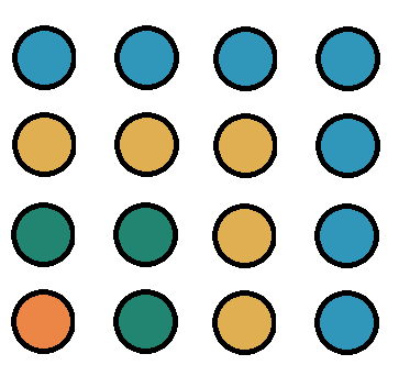
Consider the image that shows 16 colored disks arranged as a square. By starting at the lower left corner of the square and grouping disks of the same color, we can count the total number of disks in the figure as follows. \begin{equation} \begin{aligned} 1 {} & = 1^{2} \\ 1 + 3 {} & = 4 = 2^{2} \\ 1 + 3 + 5 {} & = 9 = 3^{2} \\ 1 + 3 + 5 + 7 {} & = 16 = 4^{2} \\ \end{aligned} \end{equation}
Notice that the sum of the odd integers on the left-hand side of each equation is equal to the square of the number of odd integers on the left-hand side of the equation. This means that the predicate \[P(n)\text{: "The sum of the first } n \text{ positive odd integers is equal to } n^{2} \text{."}\] is a True statement for the natural numbers \(n \in \{ 1, 2, 3, 4 \},\) that is, each of the following four propositions is True:
-
\(P(1)\): "The sum of the first \(1\) positive odd integers is equal to \(1^{2}\)." (I know this is not proper English, but please bear with me!)
-
\(P(2)\): "The sum of the first \(2\) positive odd integers is equal to \(2^{2}\)."
-
\(P(3)\): "The sum of the first \(3\) positive odd integers is equal to \(3^{2}\)."
-
\(P(4)\): "The sum of the first \(4\) positive odd integers is equal to \(4^{2}\)."
In the following code snippet, function \(P\) implements the predicate used in this example. Recall that the predicate’s output is a proposition - the output is just a string of symbols and does not indicate whether the proposition is True or False.
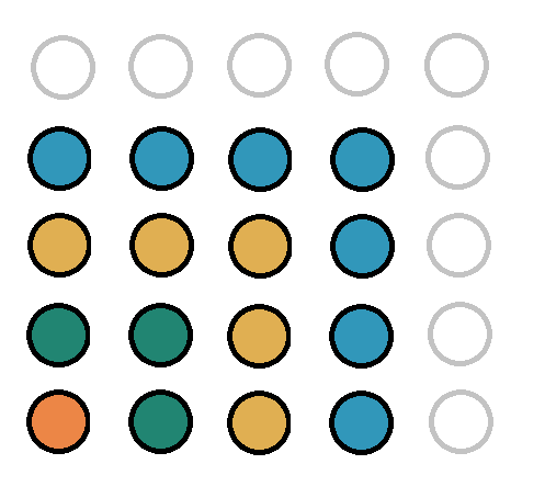
Next, consider this second image, which shows how you could change the first image to one that can be used to prove that \(P(5)\) is True.
It’s easy to show that the proposition \(P(5)\) is True because you can just write out and verify that \(1 + 3 + 5 + 7 + 9 = 25 = 5^{2}.\) The goal here is to relate the truth value of the proposition \(P(5)\) to the truth value of the “preceding proposition” \(P(4),\) in a way similar to how the numerical value of a term of a sequence can be related to the numerical value of the “preceding term” of the sequence using a recurrence relation.
Notice that the second image shows that, given the square arrangement of disks that has 4 disks along each side, we can construct a square arrangement that has 5 disks along each side by inserting 4 new disks above the top row, 4 new disks in a column to the right of the rightmost column, and 1 new disk in the upper right corner to complete the square arrangement.
In fact, there is nothing special about the number 4 in the previous paragraph: If \(k\) is any positive natural number and we have a \(k \times k\) square arrangement of disks, we can enlarge it to a \((k+1) \times (k+1)\) square arrangement of disks by inserting \(k\) disks above, \(k\) disks to the right, and \(1\) disk in the upper right corner of the \(k \times k\) square to complete the \((k+1) \times (k+1)\) square. Algebraically, we can account for the total number of disks in the \((k+1) \times (k+1)\) square by writing \[ k^{2} + k + k + 1 = (k+1)^{2} \] which is True for any natural number \(k\) (Just simplify the left-hand side and expand the right-hand side of the equation to see that the equation must be True.)
Based on this second image, we can make a conjecture that \(P(n)\) must be True for every positive natural number \(n.\) We now need to prove this conjecture.
Notice that if we combine the propositions
-
\(P(1)\) and \(P(2)\) and \(P(3)\) and \(P(4)\)
-
For all \(k \in \mathbb{N},\) \(P(k)\) implies \(P(k+1).\)
then we can build a proof for all the integers up to and including any value of \(n \in \mathbb{N}\) that we want.
For example, to prove \(P(1,\!000,\!000),\) we could start by asserting that \(P(1)\) is True, then apply the conditional \(P(k) \rightarrow P(k+1)\) along with the rule of inference modus ponens \(999,\!999\) times to prove that \(P(1,\!000,\!000)\) is True. This proof is finite - I never claimed that the proof would be short!
As an analogy,
think
of repeatedly applying modus ponens to the conditional as using a loop in code. We are just repeating the same argument \(( P(k) \land ( P(k) \rightarrow P(k+1) ) ) \rightarrow P(k+1)\) over and over again as the value of the variable \(k\) is incremented by 1 at the end of each
loop
iteration until we reach the value
that we want to stop at.
In the following code snippet, the user-defined function addTheOdds implements the computations used in this example’s argument. Notice how the Basis Step corresponds to validating the loop initialization and how the Induction Step corresponds to validating the output at the end of each loop iteration (assuming that the values were correct at the start of that loop iteration.) You can change the value of \(n\) in the code to confirm the truth value of \(P(n)\) for any integer you’d like, assuming you have enough time and computing resources.
Since we can now, in principle, build a proof of \(P(n)\) for any value of \(n \in \mathbb{N}\) that we could choose, we conclude that \((\forall \in \mathbb{N})P(n).\) That is, we have proven the proposition \[ \text{"For every positive natural number } n \text{, the sum of the first } n \text{ positive odd integers is equal to } n^{2} \text{."}\] Another way to look at this is to define \(s(n)\) to be the number of disks in a \(n \times n\) square arrangement of disks. We have shown that \(s(1) = 1\) and that \(s(k+1) = s(k) + 2k + 1\) for every positive natural number value of \(k,\) and have concluded that \(s(n) = n^{2}\) for every positive natural number \(n.\)
We will rewrite the above example more formally (with full algebraic detail) later in the chapter.
11.2. The “Proof By Mathematical Induction” Technique
A proof by mathematical induction of a predicate \(P(n)\) defined for natural numbers \(n \in \mathbb{N}\) consists of three steps.
| Basis Step |
Prove the predicate \(P(n)\) is True for some small value of \(n.\) In most but not all cases, you prove either \(P(0)\) or \(P(1).\) |
| Induction Step |
Prove that the conditional statement \(P(k) \rightarrow P(k+1)\) is True for any integer \(k.\) |
| Conclusion Step |
Conclude that \(P(n)\) is True for all natural numbers \(n\) that are greater than or equal to the smallest value used in the Basis Step. |
You can compare the first two steps of a proof by mathematical induction to the two steps used in a recursive definition as in the Sequences and Recursion chapter. Note that a recursive defintion is used to describe and define a process for constructing objects or a set of objects or a structure, but a proof by mathematical induction is used to justify and validate such a process.
Note that each of the three steps will be a proof of finite length, but will allow us to conclude that \(P(n)\) is true for every natural number \(n\) greater than or equal to some some small natural number \(b \geq 0\).
As an analogy, imagine we are building a tower using interlocking toy blocks. How tall can the tower be?
The basis step involves placing a foundation on the ground (either a flat surface for \(n = 0\), or a first block for \(n = 1\)),
and the induction step justifies that if we have built a tower that has height \(k\) then we can build a tower of height \(k+1\) by placing one more block on the tower. The conclusion step states that we can build a tower that is of any finite height \(n\) (as long as we have
enough
blocks and ignore issues arising from real-world physics!) Note that we never build an infinitely tall tower.
Note: Some textbooks and sources use an "infinite ladder" analogy for mathematical induction, but this is not quite correct. A better analogy is a ladder that can be extended to any finite height you need, but that is always of finite height.
Let’s finish this section with an example of using this proof technique. Here is a proof of the Handshake Theorem for graphs.
11.3. The Principle of Mathematical Induction
The “proof by mathematical induction” technique is justified by the Principle of Mathematical Induction, often abbreviated as PMI.
In the Remix, the Principle of Mathematical Induction is treated as an axiom, a statement that is assumed to be True about the set of natural numbers.
This principle has been used for nearly 2,000 years, but was only formalized by mathematicians about 150 years ago. See the History section, as well as the References, at this Wikipedia page for more information.
The Principle of Mathematical Induction may seem like an “obviously True” statement. If 0 is in a set, and if for each natural number in the set the next biggest natural number is also in the set, then it would seem that you can list all the elements of the set by simply counting up by 1, starting at 0. The issue that arises is that you can never stop counting up because there are infinitely many natural numbers! Instead, mathematicians can state that they are assuming that the Principle of Mathematical Induction is True without further justification.
As another example of why PMI is assumed to be True, consider the predicate that was used in the first example of this chapter: \[P(k)\text{: "The sum of the first } k \text{ positive odd integers is equal to } k^{2} \text{."}\]
What a mathematician would really like to do is to run an infinite loop, like the one shown in the code listing below, to verify that the predicate is True for every natural number greater than or equal to 1.
def P(k):
    return f"\"The sum of the first {k} positive odd integers is {k*k}\""

def addTheOddsForever():
    sum = 1
    k = 1
    if sum != k*k:
        print(P(k),"is a False proposition.")
        return False
    while True: # loop forever...
        sum = sum + 2*k + 1
        k = k + 1
        if sum != k*k:
            print(P(k),"is a False proposition.")
            return False
    return True

if addTheOddsForever():
    print("P(n) is a True proposition for each every natural number n.")
When addTheOddsForever() returns True, the code will have verified the predicate for every positive natural number… but when will addTheOddsForever() ever return True?
We only exit the loop if the predicate is False for some value of k (that is, if we find a counterexample) but otherwise we will never exit the loop to return True! We will have to wait “forever” for the answer, which dows not help us humans much — we would run out of memory or processing power or time in the universe before that.
Since the code with the infinite loop cannot verify the predicate for all natural numbers greater than or equal to 1, the mathematician will settle for using the following code sample instead, as long as the variable stop_value can be made
larger and larger, with no upper bound on how large it can be (Again, this won’t really work due to real-world constraints, but at least it does avoid the infinite loop.)
This code can verify the predicate for all natural numbers starting from 1 up to and including stop_value. The Principle of Mathematical Induction is stating that you can justify that
the predicate \(P(k)\) is True for all positive natural numbers by instead verifying that addTheOddsRevised(stop_value) will return True for every possible positive natural number value you could assign to stop_value.
11.4. More Example Proofs Using Mathematical Induction
The next example proof is the formal proof that corresponds to the first example of this chapter.
MORE PROOFS TO COME!
11.5. Validating An Algorithm Using Induction
In this section, we’ll prove that the Euclidean Algorithm as described below correctly computes the greatest common divisor of two positive integers.
-
Task: Given the positive integers \(a\) and \(b\) with \(a > b\), compute the greatest common divisor (or "g.c.d") of \(a\) and \(b.\) That is, compute the greatest integer that is a factor of both \(a\) and \(b.\)
-
Input: Two positive integers
-
Steps:
-
Set \(a\) to the greater and \(b\) to the lesser of the two input values.
-
Compute the remainder \(r\) when \(a\) is divided by \(b\) (using long division of integers, not "floating-point" decimals.)
-
If \(r > 0\)
-
Set \(a\) equal to \(b\)
-
Set \(b\) equal to \(r\)
-
Go to step 2
-
-
Return the value stored in \(b.\)
-
-
Output: A positive integer that is a factor of both input values.
-
First, we will prove a lemma (that is, a minor theorem) that we’ll use in the induction step of the main proof.
From the lemma we can conclude that the greatest common divisor of \(a\) and \(b\) is equal to the greatest common divisor of \(b\) and \(r.\)
We are now ready to prove the main result by induction.
|
Notice that if \(a = f_{n+2}\) and \(b = f_{n+1}\) are consecutive Fibonacci numbers then the Euclidean Algorithm requires exactly \(n\) loop iterations to compute the last nonzero remainder. The French mathematician Gabriel Lamé proved in 1844 that if the Euclidean Algorithm requires \(n\) loop iterations to compute the last nonzero remainder for two given positive integer inputs \(a\) and \(b\) (with \(a>b\)) then it must be True that both \(f_{n+2} \leq a\) and \(f_{n+1} \leq b.\) A proof by induction of Lamé’s theorem is given at this Wikipedia page. The "worst-case complexity" for the Euclidean Algorithm is described at that webpage as well: The Euclidean Algorithm is \(O(log_{\phi}(b)).\) (Complexity and "big \(O\)" notation are discussed in the Rates of Growth of Functions chapter.) |
11.6. Strong Induction
Strong induction is used when it is easier to use the assumption that all the propositions \(P(0), P(1), \ldots , P(n-1)\) are True in order to prove that \(P(n)\) is True.
| Basis Step |
Prove the predicate \(P(n)\) is True for one or more consecutive small values of \(n;\) in most but not all cases, you prove both \(P(0)\) and \(P(1).\) |
| Induction Step |
Prove that the conditional statement \(( P(0) \land P(1) \land \cdots \land P(k) ) \rightarrow P(k+1)\) is True for any natural number \(k.\) |
| Conclusion Step |
Conclude that \(P(n)\) is True for all natural numbers \(n\) that are greater than or equal to the smallest value used in the Basis Step. |
In spite of the name, strong induction and "weak" induction are equivalently powerful techniques in the sense that any proposition that you can prove using strong induction can also be proven by "weak" induction, and any proposition that you can prove using "weak" induction can also be proven by strong induction. The choice of which of the two proof techniques to use is based on convenience only, not power.
Next, we’ll prove the following theorem.
11.7. Validating A Recursive Algorithm Using Strong Induction
In this section, we’ll use strong induction to prove the correctness of a recursive algorithm. That is, we will show that the algorithm must work as intended.
Strong induction is useful for proving properties of recursively-defined objects since each use of the Recursion Step can depend on any previously completed steps instead of just one previous step.
11.7.1. The MergeSort Algorithm
In this subsection, we describe the MergeSort algorithm, which is an example of a “divide-and-conquer” algorithm that breaks up a large problem into two or more smaller versions of the same problem and then combines the solutions of the smaller problems to find a solution to the original large problem.
Here is a description of the MergeSort algorithm.
-
Task: Sort the numbers in a list \(L\) in increasing order. The numbers can be integers or real numbers.
-
Input: The list \(L.\)
-
Steps:
-
If the length of list \(L\) is less than \(2,\) return \(L.\)
-
Set \(c\) to the ceiling of half the length of list \(L.\)
-
Define the list \(L_{\text{left}}\) to be the list of the first \(c\) elements of list \(L,\) in the current order, and
define \(L_{\text{right}}\) to be the list of the remaining elements of list \(L\), in the current order. -
Define \(L_{\text{sorted}}\) to be the list returned by the Merge algorithm called with the two input lists \(MergeSort(L_{\text{left}})\) and \(MergeSort(L_{\text{right}}).\)
-
Copy the values to \(L\) from \(L_{\text{sorted}}.\)
-
Return \(L.\)
-
-
Output: The list \(L,\) sorted in increasing order.
The MergeSort algorithm is recursive:
| Basis Step |
The shortest lists, ones that are either empty or have only a single element, are processed at Step 1 of the algorithm. These lists are considered to be sorted by definition. |
| Recursion |
Longer lists are processed starting at Step 2 of the algorithm. In particular, notice that at Step 4, the algorithm calls on a second algorithm, Merge, after recursively calling itself twice, once for each of the shorter lists \(L_{\text{left}}\) and \(L_{\text{right}}.\) |
Of course, we will need to describe precisely what the Merge algorithm does, which we will do below. An implementation of both the MergeSort and Merge algorithms in Python will be given, too. More detail about MergeSort, along with a different Python implementation, can be found in the Algorithms and Their Analysis chapter.
Next, we describe the Merge algorithm, which is designed to combine two ordered lists into a single ordered list.
-
Task: Create a new list \(M\) that is sorted in increasing order and contains all the numbers in two given lists of numbers, \(A\) and \(B,\) that already were sorted in increasing order.
-
Input: The lists \(A\) and \(B.\) The numbers in each list can be integers or real numbers.
-
Steps:
-
Define a list \(M\) and initialize it as the empty list.
-
Define index variables \(i\) and \(j\) and initialize both to \(0.\)
-
While there are elements in both \(A\) and \(B\) not yet appended to \(M\)
-
If \(A[i\)] is less than or equal to \(B[j\)]
-
Append \(A[i\)] to \(M\)
-
Increment \(i\) by \(1\)
-
-
Otherwise, \(B[j\)] must be less than \(A[i\)] so
-
Append \(B[j\)] to \(M\)
-
Increment \(j\) by \(1\)
-
-
-
If all the elements of \(A\) have been appended to \(M,\) then append all remaining elements of \(B\) to \(M.\)
-
If all the elements of \(B\) have been appended to \(M,\) then append all remaining elements of \(A\) to \(M.\)
-
Return \(M.\)
-
-
Output: List \(M,\) containing all the numbers in the two lists \(A\) and \(B,\) sorted in increasing order.
The following Python code implements both MergeSort and Merge. Try tracing through the code to see how it works. This code is a bit longer than most sample in this textbook, so it may be easier to view and trace it in a new tab or window by clicking on the link labeled “Edit in PythonTutor.”
Now that you have had the opportunity to see the how MergeSort and Merge work as implemented in Python, you are ready to try to prove the correctness of both algorithms.
First, let’s discuss a proof of correctness for the Merge algorithm.
Next, let’s prove the correctness of the MergeSort algorithm.
11.8. Exercises
-
Prove by induction:
-
For all \(n ≥ 1, \) \(1+2+3+\ldots+n=\displaystyle\sum_{i=1}^{n}i=\displaystyle \frac{n\left(n+1\right)}{2}\)
-
For all \(n ≥ 1, \) \(1^2+2^2+3^2+\ldots+n^2=\displaystyle\sum_{i=1}^{n}i^2=\frac{1}{6} n (n+1) (2 n+1)\)
-
For all \(n ≥ 1, \) \(1^3+2^3+3^3+\ldots+n^3=\displaystyle\sum_{k=1}^{n}k^3=\frac{1}{4} n^2 (n+1)^2\)
-
For all \(n ≥ 1, \) \({23}^n-1\) is divisible by 11.
-
-
Prove by induction that \(n^2+n = n(n+1)\) is even for all integers \(n ≥ 1\).
-
Find an appropriate \(N \in \mathbb{Z}\), and prove by induction that \(n^3 +3n^2\) is even for all \(n ≥ N\).
-
Find an appropriate \(N \in \mathbb{Z}\), and prove by induction that \(n^3 +2n\) is divisible by 3 for all \(n ≥ N\). (Hint: You may use the result \(n(n+1)\), is even for \(n\), an integer.)
-
Prove by induction that \(7\) divides \(2^{4n+2} + 3^{2n+1}\) for all nonnegative integers \(n\).
-
Prove that for any \(n ≥ 1\) and \(x ≥ 0\) that \(\left(1+x\right)^n\geq1+nx\).
-
For all \(n ≥ 5\), prove that \(n^2 < 2^n\)
-
Graph \(n!\) and \(2^n\), and then prove by induction that \( 2^n < n!\) for \(n>3\).
-
Graph \(n^3\) and \(5n+12\), and then use your graph to find an appropriate \(N \in \mathbb{Z}\) to prove by induction that \(5n+12 < n^3\) whenever \(n>N\).
-
Prove by induction that a set \(A\) with cardinality \(|A|=n\) has \(2^n\) subsets.
-
Prove by induction that there are \(3^n\) numbers in base 3 (using the digits 0 ,1, 2) made up of \(n\) digits.
-
Prove by induction that there are \(4^n\) numbers in base 4 (using the digits 0 ,1, 2, 3) made up of \(n\) digits.
-
State the principle of mathematical induction using a conditional logical statement.
-
Consider the sequence defined recursively as \[a_1=1,a_2=5, \text{ and } a_n=5a_{n-1}-6a_{n-2}\]
-
Calculate the first eight terms of the recursive sequence.
-
Prove by induction that the closed-form formula for the sequence is \(a_{n} = 3^{n} - 2^{n}.\)
(Hint: You can use the fact that \(2\) and \(3\) are the solutions of the quadratic equation \(x^{2} = 5x - 6.\))
-
-
Consider the sequence defined recursively as \[a_1=1 \text{ and } a_n=2a_{n-1}+n\]
-
Calculate the first eight terms of the recursive sequence
-
Prove by induction that the recursive sequence is given by the formula \(a_n={4\cdot2}^{n-1}-n-1\).
-
-
Recall that the Fibonacci numbers are defined by the following recurrence relation: \[f_{0}=0, \, f_{1}=1, \text{ and } f_{n} = f_{n-1} + f_{n-2} \text{ for } n \geq 2.\]
-
Prove by induction that \[ f_0+f_1+f_2+\ldots+f_n= f_{n+2}-1. \]
-
Prove by induction that \[ f_0^2+f_1^2+f_2^2+ \cdots + f_n^2 =f_n \cdot\ f_{n+1}. \]
-
12. Rates of Growth of Functions
CAUTION - CHAPTER UNDER CONSTRUCTION!
NOTICE: If you are NOT enrolled in the CSC 230 course that I teach at SFSU, you probably are looking for the “public version” of the book, which I only update between semesters. The version you are looking at now is the “CSC230 version” of the book, which I will be updating throughout the semester.
This chapter was last updated on April 14, 2025.
Contents locked until 11:59 p.m. Pacific Standard Time on May 23, 2025.
You have seen that some tasks can be completed by more than one algorithm. Two questions to ask are
-
"How do you choose which algorithm to use?"
-
"Why is is it important to make such a choice?"
This chapter will discuss tools you can use to help answer these questions. In particular, ways of comparing the rates of growth of functions will allow us to compare how two algorithms perform as the size of their input increase with no upper bound.
Key terms and concepts covered in this chapter:
-
Complexity
-
Big-\(\Theta\) notation
-
Big-\(O\) notation
12.1. Complexity of Algorithms
In order to implement an algorithm, there are issues of the space needed to do the work and the time needed to complete all the steps.
For example, imagine that you are asked to complete a few Algebra homework exercises by hand, and each exercise involves solving linear equations by hand using paper and pencil. Now suppose that "few" means "one hundred" and that each linear equation involves multiple steps to solve like the one below. \[ \text{Exercise 1. Solve for } x \text{: } 40(x+6)-9(3x+5) = 65(x+7)-(7x+132)\] It is not difficult to solve linear equations like this one because it is clear what steps you need to use… but it is tedious and will likely require a lot of paper! That is, it will consume a lot of time and space to solve even the first one of these equations, and you’ll have only ninety-nine more to do after that!
In this textbook, the focus will be on time complexity and asymptotics, that is, the comparison of the time needed by the algorithms as the size of the input becomes larger and larger without any bound.
12.2. The Order of a Function and Big Theta Notation
In this section, we will define a relation that describes what it means to say that "two functions grow at the same rate." More precisely, "two functions grow at the same rate, asymptotically, as the input variable grows without an upper bound." We will also introduce big \(\Theta\) notation.
Note: \(\Theta\) is the uppercase Greek letter "Theta."
Suppose that \(f\) and \(g\) are two functions, both having domain \(\mathbb{R}\) and codomain \(\mathbb{R}\). Define the relation f has the exact same order as g to mean that
The constants \(A,\) \(B,\) and \(x_{0}\) are called witnesses: The constants confirm the "has the exact same order as" relationship between the two functions.
The Remix’s definition of "has the exact same order as" is based on notations and descriptions proposed by Donald Knuth in the 1976 letter "Big Omicron and Big Omega and Big Theta" published in ACM SIGACT News.
Consider the functions \(f\) and \(g,\) each with domain \(\mathbb{R}\) and codomain \(\mathbb{R},\) described by the rules \[ f(x) = x + \sin(x), \, g(x) = x.\] The function g is linear and the function f is not, but f can be thought of as asymptotically linear in the sense that its growth is more like that shown in a straight line plot of a linear function than, say, a parabolic plot for a quadratic function or a square root function. This is what we are describing with the relation "has the exact same order as."
Let’s plot the graphs of f and two constant multiples of g to illustrate what the relation "has the exact same order as" means.
The preceding image shows the plots of the graphs of the functions \(f,\) \(0.9g,\) and \(1.1g.\) Notice that for x between -10 and 10, the corresponding y output for f is sometimes between the two straight lines, sometimes above both lines, and sometimes below both lines.
However, if we zoom out, it appears that the plotted graph of \(f\) lies between the two straight lines for all values of the input x that have a large absolute value. In fact, the image seems to indicate that \[ 0.9g(x) \leq f(x) \leq 1.1g(x) \text{ for all } x \geq 100.\]
That is, the image suggests that f has the exact same order as g.
Notice that we could prove, more rigorously, that the inequality is true, by using some algebra and the fact that the sine function’s outputs are in the interval \([-1, \, 1\)], so the functions have the exact same order. The two functions \(f\) and \(g\) grow at the same rate, asymptotically, as the input variable grows without an upper bound.
It appears from the zoomed-out plot that we could choose a value less than 100 for the bound \(x_{0},\) but the definition of "has the exact same order as" does not require us to find optimal values of any of the constants \(A,\) \(B,\) and \(x_{0}.\) In fact, if there exists at least one ordered triple \(( A, \, B, \, x_{0})\) that witnesses the "has the exact same order as" relation between two functions, then there must be infinitely many other ordered triples that witness the same relationship. As an example, we’ve used the ordered triple \(( 0.9, \, 1.1, \, 100)\) for the two multipliers and the lower bound for inputs, but we could use the same two multipliers and any value greater than 100 for \(x_{0}\) instead. Also, the triple \(( \frac{1}{4}, \, 4, \, 0)\) witnesses the same relationship since \[ \frac{1}{4}g(x) \leq f(x) \leq 4g(x) \text{ for all } x \geq 0.\]
We have the following theorem about the "has the exact same order as" relation.
These three properties let you conclude that the "has the exact same order as" relation is an equivalence relation, so the relation partitions the set \(S = \{ f \, | \, f \text{ is a function with domain and codomain } \mathbb{R} \}\) into disjoint sets. For each function \(g \in S\) we can define \(\Theta(g)\) to be the equivalence class \[ \Theta(g) = \{ f \, | \, f \text{ has the exact same order as } g \} \] Every function with domain and codomain \(\mathbb{R}\) is an element of at least one of the \(\Theta(g)\) and for any two functions \(g\) and \(h,\) the sets \(\Theta(g)\) and \(\Theta(h)\) must either be equal or have empty intersection. For example, the earlier example shows that \(\Theta(x + \sin x)\) and \(\Theta(x)\) are the same set, so we can say that the function \(f(x) = x + \sin x\) is of linear order.
|
Mathematicians and computer scientists are very different beasts… well, they are all human but they have developed different cultures so they often use the same symbols in different ways. A mathematician, like the author of the Remix, would write the very formal \(f \in \Theta(g)\) and state "f is an element of Theta g" to mean that "f has the exact same order as g." In the earlier example, a mathematician could abbreviate this a little bit and write "\(x + \sin(x)\) is in \(\Theta(x).\)" Computer scientists have traditionally written this relation as \(f(x) = \Theta(g(x))\) and state "\(f(x)\) is big Theta of \(g(x)\)." In the earlier example, a computer scientist could write "\(x + \sin(x) = \Theta(x)\)." As a mathematician, I need to point out that the function f is not equal, in the mathematical sense, to the equivalence class containing g because it’s just one of the infinitely many functions in that equivalence class. I believe that both mathematicians and computer scientists agree that Θ(g(x)) = f(x) is just too hideous a notation to use… so please do not ever, ever use it! |
12.3. Big O notation
Traditionally, computer scientists are much more interested in the idea that "f grows at most at the rate of g". This corresponds to the second part of the inequality used to define big Theta in the previous section.
Note that Big O only gives an upper bound on the growth rate of functions. That is, the function \(f(x) = x + \sin(x)\) with domain and range \(\mathbb{R},\) used in an earlier example, is \(O(x)\) but also is \(O(x^{2})\) and is \(O(2^{x}).\)
Big O is typically used to analyze the worst case complexity of an algorithm. If, for example, \(n\) is the size of the input, then big O really only cares about what happens in the "worst-case" when \(n\) becomes arbitrarily large. Mathematically, we want to consider time complexity in this asymptotic sense, when \(n\) is arbitrarily large, so may ignore constants. That we can ignore constants will make sense after discussing how limits, borrowed from continuous mathematics (that is, calculus), can be used to compare the rates of growth of two different functions.
12.3.1. Common Complexities To Consider
The size of the input complexities most commonly used, ordered from smallest to largest, are as follows.
-
Constant Complexity: \(O(1)\)
-
Logarithmic Complexity: \(O(\log (n))\),
-
Radical complexity : \(O(\sqrt{n})\)
-
Linear Complexity: \(O(n)\)
-
Linearithmic Complexity: \(O(n\log (n))\),
-
Quadratic complexity: \(O(n^2)\)
-
Cubic complexity: \(O(n^3)\),
-
Exponential complexity: \(O(b^n)\), \( b > 1\)
-
Factorial complexity: \( O(n!)\)
To understand the sizes of input complexities, we will look at the graphs of functions; it is easier to consider these functions as ones that are defined for any real value input instead of just the natural numbers. This will also allow us to use continuous mathematics (that is, calculus) to analyze and compare the growth of different functions.
Radical growth is larger than logarithmic growth:
| In the preceding graph, we’ve used \(\text{Log}[x\)] to label the graph of a logarithmic function without stating the base for the logarithm: Is this the function \(y = log_{2}(x)\), \(y = log_{10}(x)\), \(y = ln(x) = log_{e}(x)\), or a logarithm to some other base? For the purposes of studying growth of functions, it does not matter which of these logarithms we use: You may recall that one of the properties of logarithms states that for two different positive constant bases \(a\) and \(b\) we must have \(log_{a}(x) = log_{a}(b) \cdot log_{b}(x)\), where \(log_{a}(b)\) is also a constant. As stated earlier, we may ignore constants when considering the growth of functions. |
Polynomial growth is larger than radical growth:
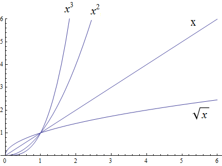
Exponential growth is larger than polynomial growth:

Factorial growth is larger than exponential growth:
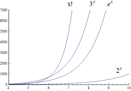
| In the preceding graph, we’ve used \(x!\) to label the graph of the function \(y = \Gamma(x+1)\) , where \(\Gamma\) is the Gamma function which is defined and continuous for all nonnegative real numbers. That is, \(n! = \Gamma(n+1)\) for every \(n \in \mathbb{N}\). Further study of the Gamma function is beyond the scope of this textbook. |
Using the graphical analysis of the growth of typical functions we have the following growth ordering, also presented graphically on a logarithmic scale graph.
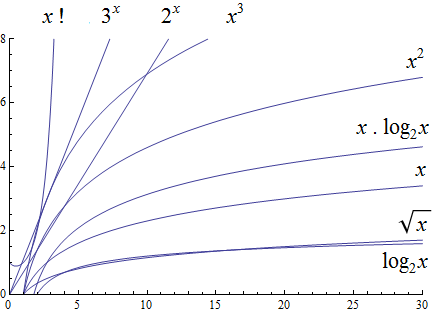
The asymptotic behavior for large \(n\) should be determined by the most dominant term in the function for large \(n\). For example, \(f(x)=x^{3} + 2x^{2}-2x\) for large \(x\), is dominated by the term \(x^3\). In this case we want to state that \(f(x)=O(x^3)\). For example \(f(1000) =1.001998×10^9≈ 1×10^9 =1000^3\). For large \(x\), \(f(x) ≈x^3\) or asymptotically, \(f(x)\) behaves as \(x^3\) for large \(x\). We write \(f(x)=O(x^3),\) that is, \(x^3 +2x^2-2x=O(x^3).\)
Likewise we want to say that if \(c\) is a constant that \(c \cdot f(x)\), and \(f(x)\) have the same asymptotic behavior for large \(n\), or \(O(c \cdot f(x))=O(f(x))\).
Show that \(f\left(x\right)=2x^2 +4x\) is \(O(x^2)\)
While intuitively we may understand that the dominant term for large \(x\) is \(x^2\) so that \(f(x) = O\left(x^2\right)\), we show this formally by producing as witnesses \(A=3\) and \(n =4\) with reference to the following graph.
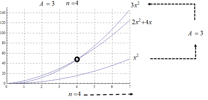
Show that \(f(x) =2x^3 +3x\) is \(O(x^3)\), with \(A=3\) and \(n=2\). Support your answer graphically.
Notice that \( x^3 > 3x\) when \( x \geq 2\). This means \(2x^3 +x^3 > 2x^3 +3x \) when \(x >2 \). In other words \( 3x^3 > 2x^3 +3x\) whenever \( x>2\), confirming \(A=3\) and \(n=2\) as witnesses, and supported by the following graph.
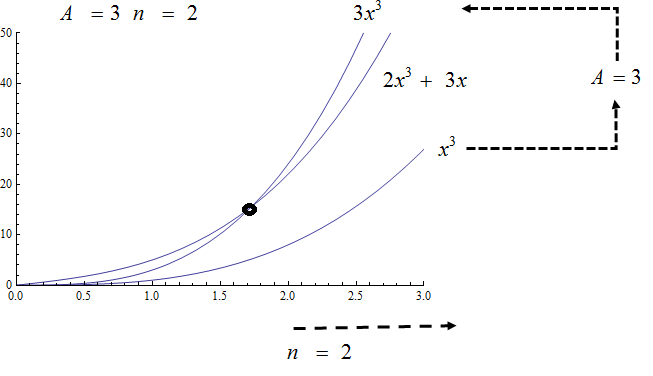
To show that a function \( f(x)\) is not \(O(g(x))\), means that no \(A\) can scale \(g(x)\) so that \( Ag(x) \geq f(x)\) for \(x\) large enough as in the following example.
Show that \( f(x) = x^2\) is not \( O( \sqrt{x})\).
Consider the graphs of \( \sqrt{x}\), \( 2 \sqrt{x}\), \( 3\sqrt{x}\), and the graph of \(x^2\). Notice that eventually, or for \(x\) large enough, \(x^2\) is larger than any \(A \sqrt{x}\) as in the figure below
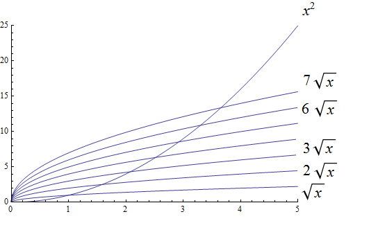
Suppose \(A>1\) is given and fixed, then if \( f(x) = x^2\) is \( O(g(x))=O( \sqrt{x})\) , there is a corresponding \(n\), also fixed, for which \(A \sqrt{x} \geq x^2\) whenever \(x>n\).
We solve the inequality \(A \sqrt{x} ≥ x^2\) by dividing both sides by \(\sqrt{x} =x^{1/2}\), to obtain, \(A \sqrt{x} ≥ x^{3/2}\).
But \(A\) is fixed and cannot be greater than all arbitrarily large \( x^{3/2}\). Hence no such \(n\) can exist for a given fixed \(A\).
For example, consider \(g(x)=A \sqrt{x}\) and \( f(x) =x^2 \), when \( x= A^2\) we obtain \( g(A^2) = A \sqrt{(A^2)}= A^2\) and \( f(A^2) = {\left ( {A}^2 \right )}^2\) and \( f(A^2)= A^4 > A^2 = g(A^2) \) when \(A>1\).
12.4. Properties of Big O notation.
Suppose \(f(x)\) is \(O(F(x))\) and \(g(x)\) is \(O(G(x))\).
We can use these properties to show for instance \( 2x^2\) is \(O\left(x^2\right)\). Likewise if \(f(x) =2x^2\) and \(g(x) =4x\), then \( 2x^2\) is \(O(x^2)\) and \( 4x\) is \(O(x)\), and the maximum gives that \(2x^2+4x\) is \( O(\max(x^2, x)) =O(x^2)\).
It is true in general that if a polynomial \(f(x)\) has degree \(n\) then \(f(x)\) is \(O(x^n)\).
For example, if \(f(x)= x^3+1\) being \( O(x^3)\), and \(g(x)=x^2-x\) being \(O(x^2)\), then \(f(x) \cdot g(x)\) is \(O(x^3 \cdot x^2) =O(x^5)\). This is verified explicitly by multiplying \(f(x) \cdot g(x)= (x^3+1) \cdot (x^2-x)= x^5 -x^4+x^2-x \) which clearly is \(O(x^5)\)
As a final example we consider ordering three functions by growth using the basic properties for Big O and the basic orderings.
12.5. Using Limits to Compare the Growth of Two Functions (CALCULUS I REQUIRED!)
In general, the Remix avoids using calculus methods because calculus is part of continuous mathematics, not discrete mathematics. However, it can be useful to use calculus to compare the growth of two functions \(f(x)\) and \(g(x)\) that are defined for real numbers \(x\), are differentiable functions on the interval \((0,\, \infty)\), and satisfy \(\lim_{x \to \infty} f(x) = \lim_{x \to \infty} g(x) = \infty\). To avoid needing to use the absolute value, we can assume that \(0 < f(x)\) and \(0 < g(x)\) for all \(x \geq 0\) (This assumption is safe to make since both functions go to infinity as \(x\) increases without bound, which means that both functions are positive for all \(x\) values greater than or equal to some number \(x_{0}\)… we are just assuming that \(x_{0}=0\) which is the equivalent of shifting the plots of \(f\) and \(g\) to the left by \(x_0\) units.)
If \(f(x)\) and \(g(x)\) are such functions and \(\lim_{x \to \infty} \frac{f(x)}{g(x)} = L\), where \(0 \leq L < \infty\), then \(f(x)\) is \(O(g(x)),\) and if \(0 < L < \infty\) then \(f(x)\) is \(\Theta(g(x)).\)
To see this, recall that \(\lim_{x \to \infty} \frac{f(x)}{g(x)} = L\) means that we can make the value of \(\frac{f(x)}{g(x)}\) be as close to \(L\) as we want by choosing \(x\) values that are sufficiently large. In particular, we can make \(L-\frac{L}{2} < \frac{f(x)}{g(x)} < L+\frac{L}{2}\) be true for all \(x\) greater than some real number \(x_{0}\). Now we can use the earlier stated assumption that \(0 \leq g(x)\) to rewrite the inequality as \((L-\frac{L}{2}) \cdot g(x) < f(x) < (L+\frac{L}{2}) \cdot g(x)\), which is true for all \(x >x_{0}\). We can choose for our witnesses \(B = L + \frac{L}{2}\) and \(x_{0}.\) This means that \(f(x) < B \cdot g(x)\) whenever \(x > x_{0},\) which shows that \(f(x)\) is \(O(g(x))\). Furthermore, if \(L>0\) we can choose \(A = L - \frac{L}{2}\) as a witness for the lower bound, too, which means that \( A \cdot g(x) < f(x) < B \cdot g(x)\) whenever \(x > x_{0},\) so \(f(x)\) is \(\Theta(g(x))\).
Note that using this method does not focus on determining the actual numerical values of \(A\) and \(n\) but just guarantees that the witnesses exist, which is all that is needed to show that \(f(x)\) is \(O(g(x))\).
12.6. Exercises
-
Give Big O estimates for
-
\(f\left(x\right)=4\)
-
\(f\left(x\right)=3x-2\)
-
\(f\left(x\right)=5x^6-4x^3+1\)
-
\(f\left(x\right)=2\ \ \sqrt x+5\)
-
\(f\left(x\right)=x^5+4^x\)
-
\(f\left(x\right)=x\log{x}+3x^2\)
-
\(f\left(x\right)=5{x^2e}^x+4x!\)
-
\(f\left(x\right)=\displaystyle \frac{x^6}{x^2+1}\) (Hint: Use long division.)
-
-
Give Big O estimates for
-
\(f\left(x\right)=2^5\)
-
\(f\left(x\right)=5x-2\)
-
\(f\left(x\right)=5x^8-4x^6+x^3\)
-
\(f\left(x\right)=\) \$4 root(3)(x)+3\$
-
\(f\left(x\right)=3^x+4^x\)
-
\(f\left(x\right)=x^2\log{x}+5x^3\)
-
\(f\left(x\right)=5{x^610}^x+4x!\)
-
\(f\left(x\right)=\displaystyle \frac{x^5+2x^4-x+2}{x+2}\) (Hint: Use long division.)
-
-
Show, using the definition, that \(f\left(x\right)=3x^2+5x\) is \(O(x^2)\) with \(A=4\) and \(n=5\). Support your answer graphically.
-
Show, using the definition, that \(f\left(x\right)=x^2+6x+2\) is \(O(x^2)\) with \(A=3\) and \(n=6\). Support your answer graphically.
-
Show, using the definition, that \(f\left(x\right)=2x^3+6x^2+3\) is \(O(x^2)\). State witnesses \(A\) and \(n\), and support your answer graphically.
-
Show, using the definition, that \(f\left(x\right)=\ {3x}^3+10x^2+1000\) is \(O(x^2)\). State the witnesses \(A\) and \(n\), and support your answer graphically.
-
Show that \(f\left(x\right)=\sqrt x\) is \(O\left(x^3\right)\), but \(g\left(x\right)=x^3\) is not\(\ O(\ \sqrt x)\).
-
Show that \(f\left(x\right)= x^2\) is \(O\left(x^3\right)\), but \(g\left(x\right)=x^3\) is not\(\ O( x^2)\).
-
Show that \(f\left(x\right)=\sqrt x\) is \(O\left(x\right)\), but \(g\left(x\right)=x\) is not\(\ O(\ \sqrt x)\).
-
Show that \(f\left(x\right)=\) \$root(3)(x)\$ is \(O\left(x^2\right)\), but \(g\left(x\right)=x^2\) is not \$O( root(3)(x))\$
-
Show that \(f\left(x\right)=\) \$root(3)(x)\$ is \(O\left(x\right)\), but \(g\left(x\right)=x\) is not \$root(3)(x)\$.
-
Order the following functions by growth \(x^\frac{7}{3},\ e^x,\ 2^x,\ x^5,\ 5x+3,\ 10x^2+5x+2,\ x^3,\log{x,\ x^3\log{x}}\)
-
Order the following functions by growth from slowest to fastest. \(\ 3x!,\ {10}^x,\ x\cdot\log{x},\ \log{x\cdot\log{x,\ \ }2x^2+5x+1,\ \pi^x,x^\frac{3}{2}\ },\ 4^5,\ \ \sqrt{x\ }\cdot\log{x}\)
-
Consider the functions \(f\left(x\right)=2^x+2x^3+e^x\log{x}\) and \(g\left(x\right)=\sqrt x+x\log{x}\). Find the best big \(O\) estimates of
-
\((f+g)(x)\)
-
\((f\cdot\ g)(x)\)
-
-
Consider the functions \(f\left(x\right)=2x+3x^3+5\log{x}\) and \(g\left(x\right)=\sqrt x+x^2\log{x}\). Find the best big \(O\) estimates of
-
\((f+g)(x)\)
-
\((f\cdot\ g)(x)\)
-
-
State the definition of "\( f(x)\) is \( O(g(x))\)"" using logical quantifiers and witnesses \(A\) and \(n\).
-
Negate the definition of "\( f(x)\) is \( O(g(x))\)" using logical quantifiers, and then state in words what it means that \( f(x)\) is not \( O(g(x))\).
13. Algorithms and Their Analysis
CAUTION - CHAPTER UNDER CONSTRUCTION!
NOTICE: If you are NOT enrolled in the CSC 230 course that I teach at SFSU, you probably are looking for the “public version” of the book, which I only update between semesters. The version you are looking at now is the “CSC230 version” of the book, which I will be updating throughout the semester.
This chapter was last updated on November 16, 2025.
added closed-form solution for the recurrence relation that describes the number of comparisons used by the MergeSort algorithm for lists of length a power of 2.
An algorithm is a step-by-step process, defined by a set of
instructions to be executed sequentially, that is used to compute a value or solve a problem. Algorithms are used in discrete mathematics to perform numerical computations, to sort lists, to do searches, insertions, and deletions of items in data structures, to solve optimization problems, and more.
The word algorithm is derived from the name of Abū ‘Abd Allāh Muḥammad ibn Mūsā al-Khwārizmī. Western Europeans learned how to do arithmetic with Hindu-Arabic numerals and the base-ten place-value system from a 12th-century AD Latin translation of one of al-Khwārizmī’s books
(The Latin translation was done about 300 years after al-Khwārizmī wrote the original book in Arabic; the original is now lost.)
By the way, the word algebra is derived from the title of another one of Al-Khwārizmī’s books.
| In this chapter, several algorithms are implemented in Python using non-optimal code to illustrate all steps needed. As mentioned in the About this text chapter, this was a deliberate choice because the code examples are designed for teaching the mathematical concepts and for neither presenting the most efficient implementations nor illustrating the "Pythonic" way of coding. However, a few code examples in this chapter do show how you can complete the same task by using some of Python’s built-in methods. |
Key terms and concepts covered in this chapter:
-
Algorithm
-
Properties of an algorithm
-
-
Types of algorithm
-
Arithmetic
-
Search
-
Sorting
-
13.1. What Is An Algorithm? What Is Not An Algorithm?
There are several problem-solving strategies that humans use, but not all of these strategies are algorithms.
An algorithm should have the following properties, based on Donald E. Knuth’s description in his famous Art of Computer Programming, The: Volume 1: Fundamental Algorithms, 3rd Edition:
| Definiteness |
Each step must be precisely defined. The actions taken at each step must be unambiguously specified. |
| Effectiveness |
Each step must be so basic that it can be done exactly and in a finite length of time. |
| Finiteness |
The process must terminate after a finite number of steps (although the number of steps may be a very large natural number.) |
| Input |
Zero or more input quantities are taken from a specified set. Inputs can be introduced before the initial step of the algorithm or dynamically before any later step of the algorithm. |
| Output |
The algorithm produces one or more outputs that have a specified relation to the inputs. Furthermore, the algorithm should produce the correct outputs for each set of inputs. |
13.1.1. An Example: Finding the Minimum in a List of Integers
Consider the following algorithm for finding the minimum element in a finite sequence of integers.
-
Task: Given a finite list of integers, find then minimum value in the list.
-
Input: A finite list of integers L.
-
Steps:
-
Define a variable \(min\) and set its value to the initial value in the list.
-
While there are values in the list that have not been examined,
-
Increase the index by 1
-
If the value of the element at the current index is less than the value of \(min,\) set the value of \(min\) to the value of the element at the current index.
-
-
-
Output: The value of \(min.\)
Does this satisfy all the requirements for an algorithm? Each step is precisely defined and can be done exactly and in a finite length of time. The process terminates after a finite number of steps (when \(min\) has been compared to the element at the highest index of the list.) The input and output are specified. This process satisfies the requirements for an algorithm.
A Python implementation of this algorithm is given below.
Note that Python provides a built-in function to find the minimum of a list: The minimum value of the list L can be computed using min(L).
13.2. Arithmetic Algorithms
Historically, algorithms first arose as ways to solve arithmetic problems. In this section, algorithms for such operations are presented.
13.2.1. Division By Repeated Subtraction
A simple division algorithm is presented in this subsection.
Big-O Analysis Of Division By Repeated Subtraction
Notice that the "division by repeated subtraction" algorithm has a worst-case scenario when the divisor b equals 1. In this worst-case scenario you must subtract the divisor \(b=1\) exactly \(a\) times to exit the loop, so "division by repeated subtraction" is \(O(a),\) that is, of at least linear order in the larger number \(a.\)
13.2.2. Long Division Of Natural Numbers
You can revise the previous algorithm to work faster by using place-value thinking.
Big-O Analysis Of Long Division
The worst-case scenario corresponds to the divisor \(b=1,\) which requires you to shift as many times as there are binary digits in \(a.\) Notice that \(a\) is bounded above by 2 raised to the number of binary digits; this means that
the long division algorithm is \(O(\log (a)).\)
Python provides built-in operators to find the quotient and remainder for variables a and b of type int: a//b is the quotient and a%b is the remainder. There is also the operator divmod(a,b) that returns an ordered pair (of data type tuple) containing both the quotient and the remainder, but divmod is less efficient than // and % and should only be used when you need to find both the quotient and the remainder.
|
13.2.3. Greatest Common Divisors: The Euclidean Algorithm
It is often needed to find a common divisor of two integers. This next algorithm goes back to Euclid.
Big-O Analysis Of The Euclidean Algorithm
The Euclidean Algorithm takes two positive integer inputs \(a\) and \(b\) with \(a > b.\) It can be proven using mathematical induction that the worst-case scenario for this algorithm is \(O(\log (b)).\) The proof uses the closed-form for the Fibonacci numbers.
Python’s math module includes a function gcd that will compute the greatest common divisor of two or more integers.
|
13.3. Search Algorithms
In the first two subsections you will see two algorithms for searching for a target integer within a list of integers. In the third subsection, Python’s built-in search methods are discussed.
RECOMMENDATION: The "Algorithms and Recursive Functions" activity can replace one or both of the first two subsections.
13.3.1. The Linear Search Algorithm
Linear search compares a target integer, t, to each element in a list of distinct integers, starting at index 0, and returns either the index i at which the target integer was found or a value indicating that the target integer was not found in the list.
A Python implementation of the linear search algorithm is given below.
Big-O Analysis of Linear Search
The linear search algorithm iterates across a list of \(n\) data elements. If the first element in the list is the target element, the algorithm stops. Otherwise, move to the next element and continue repeatedly until the target element is found or not. If the target element is not in the search list the algorithm exhaustively searches through every single element.
This is the worst case scenario with linear search in which the algorithm inspects every single element, either because the target element is the last element of the array, or the target element is not actually in the search list at all. The algorithm runs in \(O(n)\) time in the worst case.
13.3.2. The Binary Search Algorithm
The binary search algorithm searches a sorted list L of integers for a target value t. The algorithm starts looking for t in the middle of the sorted list. If t is greater than the value in the middle, the algorithm continues the binary search in the upper half of the list, otherwise the algorithm continues the binary search in the lower half of the list. The algorithm continues in this way until we reach a list of length 1 that either does or does not have t as its only element.
Big-O Analysis of Binary Search
The binary search algorithm searches for a target element \(x\) in a list of \(n\) elements by comparing the middle element in the the sorted data set with the target \(x\). The algorithm stops if the middle element \(a_m\) is the target element. Otherwise the search continues with half the data set—the half to the left if the middle element is larger than the target \(x\) or the half to the right if the middle element is smaller than the target.
The number of steps in the binary search then is the number of times we have to split the data set until we locate the target element, or determine that the target element is not in the search list after splitting down to 1 element.
The number of times we need to split the data set of size \(n\), in the worst case then, is \(p\) which is found by solving the exponential equation,
\(2^p = n\).
The algorithm then is \(O(p)\).
The solution of the exponential equation, \(2^p = n\), is in log form,
\(p=\log_2{n}\).
The binary search algorithm then is \(O(p)=O(\log{n})\).
13.3.3. Searching Within a List using Python
In this subsection you will see how to use Python to efficiently search lists.
13.4. Sorting Algorithms
In this section you will see three algorithms for sorting a list of real numbers. Two of these algorithms, bubble sort and insertion sort, are inefficient but are presented here as in many other textbooks because they are easy to understand and analyze. The third algorithm, merge sort, is an efficient recursive algorithm.
| In Python, the elements of a list L can be sorted into increasing order by calling the list.sort() method. This built-in method uses one of two sorting algorithms that won’t be discussed in this textbook: the Timsort algorithm in Python versions 2.3 to 3.10, or the Powersort algorithm in Python versions 3.11 to 3.12 (the current version as of this writing). |
13.4.1. Bubble Sort

The bubble sort algorithm is a simple sorting procedure. It is typically used to sort
a
list of n data elements in either increasing or decreasing order.
NOTE: This algorithm is called "bubble sort" because "the lighter items bubble up to the top" of the list, closer to index 0, like bubbles in a drink.
WARNING: The bubble sort algorithm
produces the correct result but is
very inefficient. You should almost never use bubble sort in code that you write. In almost every application that requires sorting a list, there is an algorithm that can be used that is much more efficient than bubble sort.
You have been warned!
In fact, most modern programming languages have built-in sort methods for you to use; these built-in methods are implemented using efficient algorithms.
We describe the bubble sort algorithm for arranging a list of \(n\) real numbers in increasing order.
-
The algorithm compares the first two elements of the list and swaps them if they are out of order.
-
It continues by traversing the list in order of increasing index, comparing each pair of adjacent elements and swapping them if they are out of order until we reach the last entry in the list at index \(n-1\).
-
The last entry in the list will then be the largest element of the original list.
-
After the largest element has been sorted into position \(n-1\), the algorithm continues by again comparing the first two elements and swapping if they are out of order.
-
Continue traversing the list and comparing and swapping adjacent elements that are out of order until position \(n-2\) of the array, after which the 2nd largest element is at index \(n-2\). The elements, now at indices \(n-1\) and \(n-2\) are sorted.
-
Continue to sort at indices \(n-3,\) then \(n-4,\) and so on, until all elements are in increasing order.
A Python implementation of the bubble sort algorithm is given below.
Big-O Analysis of Bubble Sort
We analyze the bubble sort algorithm beginning with a concrete list of size \(n=5\) and generalize the analysis.
Consider the case of a list of size \(n=5\). The naive bubble sort algorithm in this case will involve 4 passes.
In the first pass, there will be 4 comparisons and up to 4 swaps, after which the element in position 5 is in its correct position.
In the second pass, there will be 3 comparisons and up to 3 swaps, after which the element in position 4 is in its correct position.
In the third pass, there will be 2 comparisons and up to 2 swaps, after which the element in position 3 is in its correct position.
In the fourth pass, there will be 1 comparison and one possible swap , after which both the elements in positions 1 and 2 are both in their correct positions.
Adding the comparisons from each pass we obtain,
\(4+3+2+1=1+2+3+4\).
In general, if the list is of size \(n\), there will be \(n-1\) passes with swaps,
\((n-1)+(n-2)+...+2+1 = 1+2+...+(n-2)+(n-1)\).
You can use mathematical induction to prove that \[1+2+\cdots+(n-2)+(n-1)= \frac{(n-1)\cdot n}{2}\] and since \(\frac{(n-1)\cdot n}{2} =\frac{1}{2}n^2-\frac{1}{2}n\), the bubble sort algorithm is \(O(n^2)\).
13.4.2. Insertion Sort
The insertion sort works through a list and classifies two sections as sorted and unsorted.
-
The insertion sort scans through each element of the list using an outer loop with a variable, say \(i\).
-
At each stage, the list is divided into a sorted section, say the left section, and a section that is not sorted, say the right.
-
The location up to which the list is sorted, is denoted by a pointer or index, called a key.
-
At the current stage, the next element from the unsorted section, on the right, is inserted into its appropriate position in the sorted section on the left.
-
The process of inserting smaller elements in the left involves shifting, larger elements to the right, using a variable, say \(j\).
A Python implementation of the Insertion Sort Algorithm is given below:
Big-O Analysis of Insertion Sort
It is left as an exercise to verify that the insertion sort algorithm is \(O(n^2)\).
13.4.3. Merge Sort
Merge Sort is a recursive sorting algorithm. The general idea is to divide a list of length \(n\) into \(n\) sublists of length \(1\), where a list of length one is considered already sorted. Subsequently, the algorithm repeatedly merges the sublists to make sorted lists until only a single list of length \(n\) is remaining. This will be the a sorted list consisting of the elements of the original list.
The picture below illustrates this with a list of length seven.
Image credit: "Merge Sort Algorithm Diagram" by VineetKumar. This work has been released into the public domain by its author, VineetKumar at English Wikipedia. This applies worldwide.
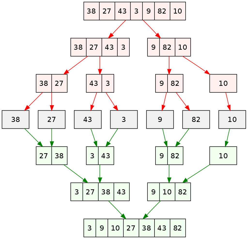
Big-O Analysis of Merge Sort
Define a function \(C(n)\) with output equal to the number of comparisons needed by Merge Sort to order a list of size \(n\). From the algorithm, you can see that \(C(n)\) satisfies the following recurrence relation. \[ C(n) = C \left( \left\lceil \frac{n}{2} \right\rceil \right) + C \left( \left\lfloor \frac{n}{2} \right\rfloor \right) + (n - 1) \] with \(C(1) = 0\) and \(C(2) = 1.\)
To simplify the analysis, let’s assume that \(n\) is a power of \(2\) so that the ceiling and floor are not needed in the recurrence relation. \[ C(n) = C \left( \frac{n}{2} \right) + C \left( \frac{n}{2} \right) + (n - 1) \] where \(n\) is a power of \(2\) and \(C(1) = 0\) and \(C(2) = 1.\) Notice that the recursive step can be rewritten as \[ C(n) = 2 C \left( \frac{n}{2} \right) + (n - 1). \] It can be shown that the closed-form solution to this recurrence relation is a function that is \(O(n \log{n}).\)
Informal exercise: Verify that \(C(n) = n \cdot \log_{2}{(n)} - (n-1)\) is a closed-form solution of the simplified recurrence relation.
MORE TO COME!
14. Graphs
CAUTION - CHAPTER UNDER CONSTRUCTION!
NOTICE: If you are NOT enrolled in the CSC 230 course that I teach at SFSU, you probably are looking for the “public version” of the book, which I only update between semesters. The version you are looking at now is the “CSC230 version” of the book, which I will be updating throughout the semester.
This chapter was last updated on November 29, 2025.
Added content to subsection on the Traveling Salesperson Problem.
Revised example involving isomophism and planarity.
Revised and expanded the discussion of isomorphisms and underlying graphs.
Graphs are discrete mathematical structures used to represent connections between individual Graphs have applications in fields such as chemistry, network analysis, computing algorithms, and social sciences.
Key terms and concepts covered in this chapter:
-
Graphs
-
Undirected graphs
-
Directed graphs
-
Weighted graphs
-
-
Creating new graphs from old graphs
-
Subgraphs
-
Unions and intersections of graphs
-
-
Graph isomorphism
-
Graph coloring
-
Connectivity of graphs
-
Eulerian circuits
-
Hamiltonian circuits
-
Shortest-path problems
-
Dijkstra’s algorithm
-
Traveling Salesperson Problem (TSP)
-
-
14.1. Introduction and Definitions
A graph consists of a set of vertices and a set of edges. Each edge connects either two different vertices or one vertex to itself. Vertices are sometimes called nodes.
-
For each edge, its endpoints are the two vertices that it connects (but notice that the “endpoints” may be the same vertex.) The edge is said to be incident with each of its endpoints.
-
An edge that connects one vertex to itself is called a loop.
-
Two edges that have the same endpoints are called parallel edges.
-
Two vertices are adjacent if they are the endpoints of at least one edge. Adjacent vertices are also called neighbors.
-
The degree of a vertex \(v\) is the number of times the vertex occurs as an endpoint for all the edges in the graph.
-
An isolated vertex is a vertex that is not an endpoint of any edge. That is, an isolated vertex is the same as a vertex that has degree 0.
-
A graph is called a multigraph if there are parallel edges in the graph.
-
A simple graph is a graph that has no loops and no parallel edges.
The following example illustrates many of these definitions.
The graph shown has 8 vertices and 7 edges.
In this drawing, the vertices are represented by points that are labeled by capital letters, and the edges are represented by the line segments and arcs that connect two vertices.
The graph is drawn so that the edge with endpoints \(B\) and \(F\) and the edge with endpoints \(D\) and \(E\) are represented by two line segments that intersect, but the point of intersection is ignored in the graph because it is not a vertex. We could redraw this graph so that the two edges do not cross; for example, we could move \(E\) inside the triangle that has vertices \(B,\) \(D,\) and \(F.\) However, there are some graphs which cannot be drawn in 2 dimensions without some edge crossings.
There is a loop: The edge that has \(D\) as both of its endpoints.
There are parallel edges that connect the vertices \(A\) and \(C,\) so this graph is a multigraph.
Vertex \(G\) is an isolated vertex - it is not an endpoint of any edge. Vertex \(H\) is also an isolated vertex.
This graph is a multigraph because there are multiple edges that connect the pair of vertices \(A\) and \(C.\)
This graph is not a simple graph: It contains a loop, and it has at least one pair of parallel edges.
Notice that in the example and definitions given so far, we’ve assumed that each edge is undirected: An edge represents a connection between its endpoints but does not indicate a direction of travel from one endpoint to the other endpoint. However, in some applications it is useful for a graph to use only directed edges that point from one endpoint to the other endpoint. A graph that has only directed edges is called a digraph, which is short for directed graph.
Most graphs discussed in this chapter will be (undirected) simple graphs, that is, graphs with no loops and no parallel edges.
14.2. The Handshaking Lemma
This section describes a property of every undirected graph.
Recall that the degree of a vertex of a graph is the number of times the vertex occurs as an endpoint for all the edges in the graph. Keep in mind that the vertex of a loop counts twice because that vertex occurs as “both endpoints” of the loop.
Consider again the graph that was drawn in the previous example.
The degrees of each of the vertices in this graph are listed in the table.
| Vertex | Degree |
|---|---|
A |
2 |
B |
2 |
C |
2 |
D |
5 |
E |
1 |
F |
2 |
G |
0 |
H |
0 |
Notice that the sum of the degrees of all the vertices is \(14\), which is equal to twice the number of edges, \(2 \cdot 7.\)
In fact, for any undirected graph with finitely many edges, the sum of the degrees of all vertices is equal to twice the number of edges (recalling that a loop’s endpoint will be counted twice.)
|
A useful consequence of the Handshaking Lemma is that the sum of the degrees of a graph must be even. |
14.3. Simple Graphs
Recall that in a simple graph, there are no loops and no parallel edges (that is, you cannot have two different edges that connect the same pair of endpoints.) This means that for a simple graph, each edge is determined by its two distinct endpoints. This allows us to give a relatively simple but formal set-theoretic definition of “simple graph.” Graphs discussed in this textbook are assumed to be simple unless stated otherwise.
14.3.1. A Formal Definition of Simple Graph
This subsection presents a formal set-theoretic definition of simple graphs.
A simple graph \(G=\left(V,\ E\right)\) is an ordered pair consisting of a nonempty set \(V\) and a (possibly empty) set \(E,\) where each element of \(E\) must be of the form \(\left\{x,y\right\}\), where \(x\) and \(y\) are two different elements of \(V.\) The elements in set \(V\) are called the vertices (or nodes) of the graph. The elements in set \(E\) are called the edges of the graph.
The graph shown has vertex set \(\left\{A,\ B,\ C,\ D,\ E,\ F\right\}\) and edge set \( \{\{A,C\},\{A,D\},\{B,D\},\{B,F\},\{C,F\},\{D,F\},\{E,F\}\}.\)
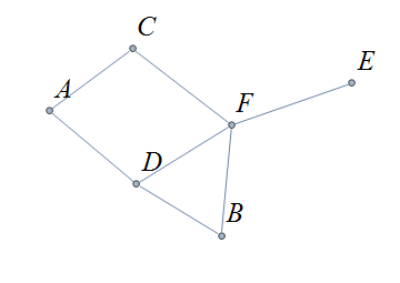
The degrees of each of the vertices in the undirected graph \(G\) with vertex set \(V=\{A,B,C,D,E,F,G\}\) and edge set \(E=\{\{A,C\},\{A,D\},\{B,D\}\{B,F\},\{C,F\},\{D,F\},\{F,G\}\}\) are,
\(d\left(A\right)=2\)
\(d\left(B\right)=2\)
\(d\left(C\right)=2\)
\(d\left(D\right)=3\)
\(d\left(E\right)=0\)
\(d\left(F\right)=4\)
\(d\left(G\right)=1\)
14.4. Directed Graphs
The main focus of this chapter will be undirected simple graphs, but we will briefly discuss directed graphs in this section.
A directed graph (or digraph) is a graph in which the edges are directed from one vertex to another vertex. Each edge has an initial vertex \(u\) and a terminal vertex \(v;\) the edge is drawn as an arrow pointing from \(u\) to \(v.\)
The out-degree of a vertex \(w\) is the number of edges that have \(w\) as the initial vertex. The in-degree of a vertex \(w\) is the number of edges that have \(W\) as the terminal vertex.
The directed graph shown has vertex set \(\{A,B,C,D,E,F\}\) and edge set \(\{ (A,C),(D,A),(B,D),(F,B),(C,F),(D,F),(F,E) \}\). The first coordinate of each edge is the initial vertex and the second coordinate is the terminal vertex.
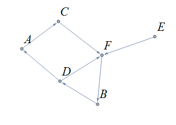
Notice that the directed edges of this graph connect the same endpoints as the undirected edges of the graph in this earlier example. The undirected graph is referred to as the underlying graph of the directed graph.
The graph \(G=(V,E)\) with vertex set \(V = \{ \text{"rock", "paper", "scissors"} \}\) and edge set \(E = \{ \text{("rock", "paper"), ("paper", "scissors"), ("scissors", "rock")} \}\) can be used to represent the game "rock, paper, scissors."
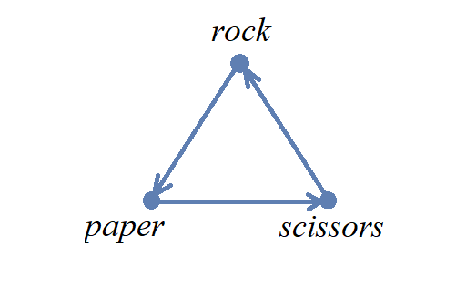
Each directed edge has for its initial vertex the loser and for its terminal edge the winner.
14.4.1. Simple Directed Graphs: A Formal Definition
We can give a formal set-theoretic definition of simple directed graph as well. To indicate the directed edges, ordered pairs of vertices are used instead of 2-element sets.
A simple directed graph \(G=\left(V,\ E\right)\) is an ordered pair consisting of a set \(V\) of objects called vertices (or nodes) and a set \(E\) of objects called directed edges. Each directed edge \(e\in\ E\) is an ordered pair of the form \(e=\left(x,y\right)\), where \(x\) and \(y\) are two different vertices in set \(V.\) For the directed edge \(e=\left(x,y\right),\) \(x\) is the initial vertex of \(e\) and \(y\) is the terminal vertex of edge \(e\).
14.5. Examples of Simple Graphs
In this section presents several classes of graphs.
The complete graph \(K_n\) is the simple graph with \(n\) vertices such that any two vertices are adjacent, that is, every pair of vertices are the endpoints of an edge. The image shows \(K_{4},\) the complete graph on 4 vertices. Click here to see images of \(K_{n}\) for the positive integers that are less than or equal to \(12.\)
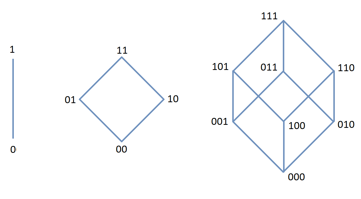
The n-cube \(Q_{n}\) can be described as the graph that has vertex set consisting of the \(2^{n}\) bitstrings of length \(n,\) and edges such that two vertices are adjacent if and only if the bitstrings differ in exactly one bit position. The image shows the three graphs \(Q_{1},\) \(Q_{2},\) and \(Q_{3};\) these graphs can be used as a way to represent the power sets of sets that have \(1,\) \(2,\) and \(3\) elements, respectively. Notice that \(Q_{2}\) can be drawn as a square and that \(Q_{3}\) can be represented as a cube in \(3\)-dimensional space (or by a drawing of a cube in a \(2\)-dimensional plane.)
A bipartite graph is a simple graph whose set of vertices can be partitioned into two disjoint nonempty sets such that every vertex is in exactly one of the two sets and every edge has one endpoint in each of the two sets. One way to think of a bipartite graph is that each vertex can be assigned one of two colors so that every edge must connect vertices of different colors. Notice that \(Q_{1},\) \(Q_{2},\) and \(Q_{3}\) are all examples of bipartite graphs (Question: Is \(Q_{n}\) a bipartite graph for every natural number \(n?\) Why or why not?)
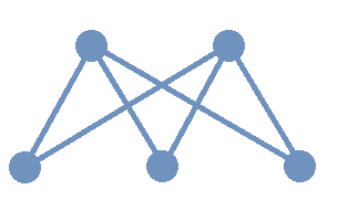
This image shows the graph \(K_{2,3}\) and is another example of a bipartite graph.
Notice that \(K_{2,3}\) has an additional property: Every pair of vertices \(\{a, b \}\) with \(a\) in the set of \(2\) "upper" vertices and \(b\) in the set of \(3\) "lower" vertices are the endpoints of an edge. A bipartite graph that has this additional property is called a complete bipartite graph. In general, the symbol \(K_{m,n}\) represents the complete bipartite graph that has two disjoint sets of vertices, one of cardinality \(|m|\) and the other of cardinality \(|n|,\) such that every pair of vertices that come from the different sets are joined by an edge. Notice that \(Q_{1} = K_{1,1}\) and \(Q_{2} = K_{2,2}\) are complete bipartite graphs, but that \(Q_{3}\) is not a complete bipartite graph because, for example, there is no edge joining \(000\) and \(111.\)
NOTE: The phrase "complete bipartite" needs to be read as a single term used to indicate that a bipartite graph has all the edges it can possibly have. For example, \(K_{2,3}\) is a bipartite graph such that if you tried to enlarge it by inserting an additional edge into the graph, that edge would join either the \(2\) "upper" vertices, \(2\) of the "lower" vertices, or \(2\) vertices that are already joined; in this sense, \(K_{2,3}\) is "complete" as a bipartite graph. \(K_{2,3}\) is not a "complete graph" in the sense of the earlier example in this section. In fact, since a "complete graph" must contain an edge for every pair of distinct vertices, the only graph that can be both a "complete graph" and a "complete bipartite graph" is \(Q_{1} = K_{2} = K_{1,1}.\) Mathematicians recycle and reuse a lot of words… .
14.6. Representing Simple Graphs
In addition to the vertex-edge drawing, a simple graph can be represented in other ways that are more useful for computing.
First, recall that if \(u\) is a vertex of a simple graph, then vertex \(v\) is said to be adjacent to \(u\) if and only if \(\{u, v \}\) are the endpoints of an edge of the graph.
One way to represent a simple graph is by using an adjacency list. This list can be written as a table, where each row has two columns. In each row, the entry in the first column is a single vertex \(v\) and the entry in the second column is a list of all vertices of the graph that are adjacent to \(v.\)
Another way to represent a simple graph is by using an adjacency matrix. The adjacency matrix of a simple graph represents the graph in table form, and contains an entry for each pair of vertices. For each vertex of the graph, there is a row and also a column. If vertices \(u\) and \(v\) are adjacent (that is, connected by some edge), then the adjacency matrix will contain a \(1\) in the position that corresponds to the row for \(u\) and the column for \(v,\) otherwise the matrix contains a \(0\) at that postion. The next example may help make this more clear.
The graph with vertex set \(\left\{A,\ B,\ C,\ D,\ E,\ F\right\}\) and edge set \(\{\{A,C\},\{A,D\},\{B,D\}\{B,F\},\{C,F\},\{D,F\},\{E,F\}\}\) can be represented by
the drawing
or the adjacency list
| Vertex | Adjacent Vertices |
|---|---|
A |
C, D |
B |
D, F |
C |
A, F |
D |
A, B, F |
E |
F |
F |
B, C, D, E |
or the adjacency matrix
\(\mathbf{M}=\left(\begin{matrix}0&0&1&1&0&0\\0&0&0&1&0&1\\1&0&0&0&0&1\\1&1&0&0&0&1\\0&0&0&0&0&1\\0&1&1&1&1&0\\\end{matrix}\right)\)
For example, in matrix \(\mathbf{M}\) the rows, from top to bottom correspond to the vertices \(A,\ B,\ C,\ D,\ E,\ F\) and the columns, from left to right, corespond to vertices \(A,\ B,\ C,\ D,\ E,\ F.\) The values in row 3, which corresponds to vertex \(C\), indicate whether the vertex for that column is adjacent to \(C.\) If we use the symbol \(M_{r,c}\) to stand for the value in row \(r\) and column \(c,\) then \(M_{3,5} = 0\) because there is no edge in the graph with endpoints \(C\) and \(E,\) and \(M_{3,6} = 1\) because there is an edge in the graph with endpoints \(C\) and \(F\).
14.7. Weighted Graphs
In some applications, each edge of a graph has a weight, which is some nonnegative number. The weight could represent the physical distance between the two endpoint nodes, or could represent the cost to travel or transmit data between the endpoint nodes.
You can use an adjacency matrix to describe a weighted graph, but instead of using a \(1\) to represent that there is an edge between two vertices you place the the weight of the edge in the correct position of the adjacency matrix, as shown in the following example.
Consider the following weighted simple graph
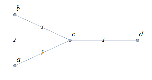
The adjacency matrix of this weighted graph is \( \left(\begin{matrix}0&2&5&0\\2&0&3&0\\5&3&0&1\\0&0&1&0\\\end{matrix}\right). \)
14.8. Creating New Graphs From Old Graphs
Given a set of one or more graphs, there are several ways to create new graphs using the graphs in the set.
14.8.1. Subgraphs
Given a simple graph \(G,\) you can form a subgraph \(H\) by choosing a subset of the vertices of \(G\) along with a subset of the edges of \(G\) such that each edge has endpoints in the set of vertices you chose. That is, \(H\) is a subgraph of \(G\) if \(H\) is a graph such that every vertex of \(H\) is a vertex of \(G\) and every edge of \(H\) is an edge of \(G.\)
More formally, \(H = (V_{H}, E_{H})\) is a subgraph of \(G = (V,E)\) if and only if all three of the following statements are True: \(V_{H} \subseteq V,\) \(E_{H} \subseteq E,\) and for every edge \(e \in E_{H}\) the endpoints of \(e\) are in \(V_{H}.\)
If \(v\) is a vertex of \(G,\) we denote by \(G-v\), the subgraph obtained from \(G\) by removing the vertex \(v\) along with all edges in \(E\) that have \(v\) as an endpoint.
The image shows a graph \(G\), and the subgraph \(G-d\) formed by removing the vertex \(d\).
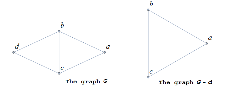
In the same way, you can obtain a subgraph by removing multiple vertices along with the edges associated with the removed vertices. The subgraph obtained is called the subgraph induced by removing those vertices.
Below is a graph \(G(V,E)\) and the subgraph obtained by \(V-\{a,d\}\), called the induced subgraph \(G-\{a,d\}\), with a slight abuse of notation
14.8.2. Unions and Intersections Of Graphs
Given two simple graphs \(G_{1}\) and \(G_{2}\), you can form the union of the graphs by taking the union of the two sets of vertices to get a new set of vertices, and taking the union of the two sets of edges to get a new set of edges. Notice that any edge that is in both graphs will only appear once in the new graph because you took the union of the sets of edges, that is, you can’t create parallel edges by forming the union.
In the same way, you can form the intersection of two simple graphs by taking the intersection of the two sets of vertices to get a new set of vertices, and taking the intersection of the two sets of edges to get a new set of edges.
14.9. Graph Isomorphism
Recall that a graph is determined by its set of vertices and how those vertices are connected by edges, but not the drawing you use to represent the graph.
Consider the two graphs shown in the image.
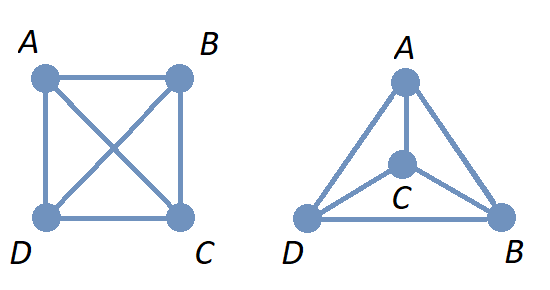
Notice that these two graphs are different-looking drawings of the same graph that has vertex set \(\{ A, B, C, D\}\) and edge set \(\{\{A,B\},\{A,C\},\{A,D\},\{B,C\},\{B,D\},\{C,D\}\}.\) Also, notice that the drawing on the left appeared earlier in the chapter, but with unlabeled vertices: Each of the graphs in the image is a drawing of \(K_{4},\) the complete graph on \(4\) vertices.
Notice that using either the adjacency list
| Vertex | Adjacent Vertices |
|---|---|
A |
B, C, D |
B |
A, C, D |
C |
A, B, D |
D |
A, B, C |
or the adajcency matrix \[\left(\begin{matrix}0&1&1&1\\1&0&1&1\\1&1&0&1\\1&1&1&0\\\end{matrix}\right)\] makes it easier to see that the two drawings represent the exact same graph.
You can imagine the graph on the right being the result of dragging the vertex \(C\) inside the "triangle" with vertices \(A,\) \(B,\) and \(D.\)
Sometimes, different graphs may be essentially the same graph, as in the next example.
Consider the two graphs, each with \(4\) vertices and \(6\) edges, shown in the image.
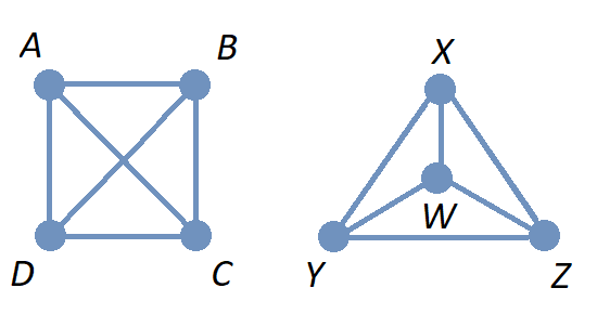
These graphs are not equal since the graph on the left has vertex set \(\{ A, B, C, D\}\) and the graph on the right has vertex set \(\{ W, X, Y, Z\}.\) However, by comparing the graph on the right to the one on the right in the previous example, you can see that there is a one-to-one correspondence between the two sets of vertices that preserves adjacency (that is, if two vertices in the upper row are endpoints of an edge of the graph on the left, then the corresponding vertices in the lower row are endpoints of an edge of the graph on the right.)
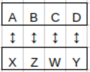
A one-to-one correspondence between the set of vertices of two simple graphs that preserves adjacency is called a graph isomorphism, and the two graphs are said to be isomorphic. That is, two vertices are endpoints of an edge in the first graph if and only if the corresponding vertices are the endpoints of an edge in the second graph. Informally, you can think of two isomorphic graphs as a pair of graphs where a drawing of one graph can be relabeled and/or reshaped to obtain a drawing of the other graph (That is, the two graphs are really the same graph but have drawings that are labeled and/or shaped differently.)
Using graph isomorphisms can help identify properties of a graph.
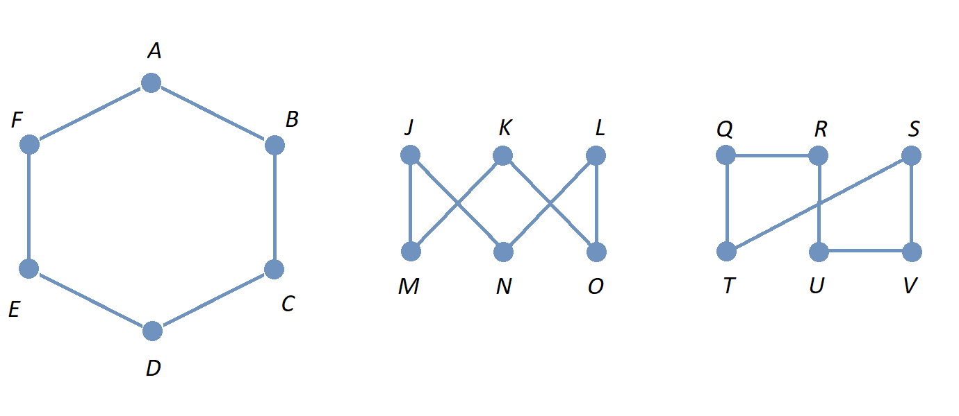
The three graphs in the image are isomorphic; it is an exercise for you to write out the one-to-one correspondences.
Write out the one-to-one correspondences between the sets of vertices that define the graph isomorphisms.
Once you have shown that the three graphs are isomorphic, you can use the fact that they are different representations of the same graph. For example,
-
It is not immediately clear that the graphs on the left and right are bipartite, but the arrangement of the vertices in the middle graph into "upper" and "lower" rows makes this easy to see.
-
Also, it is not immediately clear that the graph in the middle or the graph on the right is planar (that is, the graph can be redrawn in a \(2\)-dimension plane so that no edges cross) but this is obvious for the graph on the left.
This textbook does not discuss planar graphs in detail, but it is worth mentioning that it can be proven that neither \(K_{5}\) nor \(K_{3,3}\) is planar. If you’d like to learn more about planar graphs, one source is the section "Planar Graphs" in Oscar Levin’s Discrete Mathematics: An Open Introduction, 4th edition. |
14.9.1. Isomorphism of Graphs with Additional Features
As described above, a graph isomorphism is a one-to-one correspondence between the sets of vertices of two graphs that preserves the adjacency relationship between pairs of vertices. That is, two vertices are endpoints of an edge in one graph if and only if the corresponding vertices are endpoints of an edge in the other graph.
In cases where graphs have additional features beyond the basic adjacency relationship between pairs of vertices, we should only consider two of these “graphs with additional features” to be isomorphic if the additional features are also preserved.
Note: Some sources use the word “attributes” for these additional features.
As an example, in the image, the three graphs with vertex sets \(\{ F,\,G,\,H \},\) \(\{ J,\,K,\,L \},\) and \(\{ P,\,Q,\,R \}\) are isomorphic as graphs if we ignore the edge weights. Also, the two graphs with vertex sets \(\{ F,\,G,\,H \}\) and \(\{ J,\,K,\,L \}\) are isomorphic as weighted graphs because there is a one-to-one correspondence between the vertex sets that preserves both the adjacency relationships and the corresponding edge weights. The third graph with vertex set \(\{ P,\,Q,\,R \}\) is not isomorphic as a weighted graph to either of the other two weighted graphs because its edge weights cannot be matched with the edge weights in the other weighted graphs.
14.10. Graph Coloring
In some contexts, it can be useful to partition either the set of vertices or the set of edges of a graph into disjoint subsets to make it easier to understand the graph and the network it represents. This act of partitioning is usually referred to as "coloring" since using different colors can make it easy to see and interpret the properties of the partition when the graph is drawn. Notice that you could instead create the partition by assigning labels like "group 1," "group 2," and so on, to each vertex (or edge.)
For example, the image shows a graph called the Petersen graph with its vertex set partitioned into 3 subsets so that each edge’s endpoints are in two different subsets of the partition (That is, each edge’s endpoints have different colors.)
Image credit: "Petersen_graph_3-coloring.svg" by Д.Ильин. The copyright holder of this work has released this work into the public domain. This applies worldwide.
The next example discusses an application of vertex coloring.
The following image represents a "map" showing four countries; the blue region represents one country (not a body of water) that is surrounded by three other countries.
The map can be represented as a graph with vertices colored to match the regions, as shown on the right. If it helps you to connect the graph to the map, imagine that each vertex represents a capital city of the corresponding country.
This way of representing a map was used to prove the Four Color Theorem which states, roughly, that
Any map of countries that can be drawn in a plane such that
(1) every country has a color and
(2) no two adjacent countries have the same color
requires at most four different colors.
In this context "two adjacent countries" share a border that is not just a single point.
The first proof of the theorem was announced in 1976, and a corrected version of the first proof was published in 1989 after some errors were fixed (Yes, professional mathematicians do make mistakes!) The proof was considered controversial by many mathematicians at the time because it was the first major computer-assisted proof: Over one thousand five hundred different cases needed to be checked!
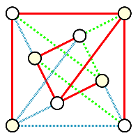
In other contexts, it is more appropriate to use edge coloring. That is, each edge of the graph is assigned a color so that the set of edges is partitioned into disjoint subsets.
For example, the graph in the image shows that the complete bipartite graph \(K_{4,4}\) can be partitioned as a union of 3 disjoint graphs called forests (Forests are defined later in this textbook, in the Trees chapter.)
Image credit: "K44 arboricity.svg" by David Eppstein. The copyright holder of this work has released this work into the public domain. This applies worldwide.
14.11. Connectivity of Undirected Graphs
A walk on a graph \(G=\left(V,E\right)\) is a finite, non-empty, alternating sequence of vertices and edges of the form, \(v_0e_1v_1e_2\ldots e_nv_n\), with vertices \(v_i\in V\) and edges \(e_i\in E\), where for each integer value of \(i \leq n\) the endpoints of \(e_i\) are the vertices \(v_{i-1}\) and \(v_i.\) The integer \(n\) is called the length of the walk.
If we restrict ourselves to simple undirected graphs, there is at most one edge joining each pair of adjacent vertices, so a walk can be specified simply by listing the sequence of vertices \(v_0v_1\ldots v_n\) (That is, we don’t need to write down the edges.)
-
A trail is a walk that does not repeat an edge. That is, all edges in a trail are distinct.
-
A path is a trail that does not repeat a vertex (but we allow for the possibility that the initial vertex \(v_0\) and terminal vertex \(v_n\) of the path are the same vertex; When \(v_0=v_n\) the path is called a closed path or a circuit.)
-
A cycle is a closed path of length at least 1.
The distance \(d(u,v)\) between two vertices \(u\) and \(v\) in a graph \(G\) is the number of edges in a shortest path connecting them, assuming such a path exists.
In the graphs below the first shows a trail \(CFDBFE\). It is not a path since the vertex \(F\) is repeated. The second shows a path \(CADFB\), and the third a cycle \(CADFC\). Also note the following distances, \(d(A,D)=1\), while \(d(A,F)=2\), and \(d(A,E)=3\).
14.12. Connected Graphs
A graph \(G\) is connected if there is a path between any pair of vertices.
The graph \(G\) below is not connected since, as just one example, there is no path between vertex \(a\) and vertex \(e.\)
\(G\) has adjacency matrix
\( \left(\begin{matrix}0&1&1&0&0\\1&0&1&0&0\\1&1&0&0&0\\0&0&0&0&1\\0&0&0&1&0\\\end{matrix}\right). \)
In the previous example, the graph \(G\) can be treated as a union of two connected subgraphs, called the connected components of \(G.\) It can be proven by mathematical induction that any simple undirected graph that has a finite number of vertices can be written as a union of a finite number of connected components.
14.13. Eulerian Graphs
An Euler path on a graph is a path that uses each edge of the graph exactly once.
An Euler circuit (also called an Eulerian trail) is a closed trail containing each edge of the graph \(G\) exactly once and returning to the start vertex. A graph with an Euler circuit is called Eulerian or is said to be an Eulerian graph.
In the following, the first graph is Eulerian. The sequence of edges \(e_1 e_2 e_3 e_4 e_5 e_6 e_7\) describes an Euler circuit (Notice that some vertices are visited multiple times; it is the edges that must appear exactly once in an Euler path.) The second graph is not an Eulerian graph. Convince yourself of this fact by looking at all necessary trails or closed trails.
The following are useful characterizations of graphs with Euler circuits and Euler paths and are due to Leonhard Euler
Euler solved a famous problem about the seven bridges of Königsberg by representing the problem as a graph (with parallel edges.)
14.14. Hamiltonian Graphs
A cycle in a graph \(G\), is called a Hamiltonian cycle if every vertex, except for the starting and ending vertex, is visited exactly once.
A graph is Hamiltonian, or said to be a Hamiltonian graph, if it contains a Hamiltonian cycle.
The following graph is Hamiltonian and shows a Hamiltonian cycle \(ABCDA\), highlighted (Notice that some edges are used multiple times; it is the vertices, starting and ending vertex, that must appear exactly once in an Hamiltonian path.) The second graph is not Hamiltonian.
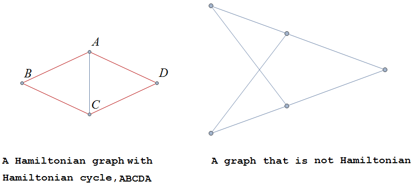
14.15. Finding A Shortest Path in a Weighted Graph: Dijkstra’s Algorithm
In some applications of graph theory, you need to find a "shortest path" between two vertices of a weighted graph. In the context, shortest may mean "of least distance" but could mean "of least cost" or something else, depending on what the edge weights represent.
Edsger Dijkstra published a paper in 1959 that describes an algorithm for finding the path of "minimum total weight" between two given vertices of a simple connected graph with weighted undirected edges.
Dijkstra’s original paper is also available in the ACM Digital Library at this link.
Here is a description of the algorithm, based on Dijkstra’s original.
-
Task: Given two vertices \(a\) and \(z,\) find the edges of a path between the two vertices that has the minimum possible sum of weights.
-
Input: The list \(V\) of all vertices of the graph, with the two vertices \(a\) and \(z\) specified, and the list \(E\) of all weighted edges of the graph.
For example, the input could be an adjacency matrix for the graph, with the first row of the matrix corresponding to \(a\) and the last row corresponding to \(z\). -
Steps:
-
Define four lists \(V_{chosen},\) \(V_{candidates},\) \(E_{chosen},\) and \(E_{candidates},\) and initialize each list as an empty list.
-
Append vertex \(a\) to the end of \(V_{chosen}.\)
-
While vertex \(z\) has not been appended to \(V_{chosen}\)
-
Set \(v\) to the last vertex appended to \(V_{chosen}.\)
-
For each vertex \(w\) that is not in \(V_{chosen}\) but is adjacent to vertex \(v\)
-
If \(w\) is in \(V_{candidates}\) and the edge \(e\) that connects \(v\) and \(w\) is part of a path between \(a\) and \(w\) that has total weight less than the weight of the known path that uses the corresponding edge in list \(E_{candidates},\) remove that edge from \(E_{candidates}\) and append \(e\) to \(E_{candidates}.\)
-
Otherwise, \(w\) is in neither list \(V_{chosen}\) nor list \(V_{candidates},\) so append vertex \(w\) to the end of \(V_{candidates}\) and append the edge \(e\) that connects \(v\) and \(w\) to the end of \(E_{candidates}.\)
-
-
After exiting the "for" loop,
-
find the vertex \(w\) in list \(V_{candidates}\) that has the minimal-weight path to the starting vertex \(a\) and append \(w\) to the end of \(V_{chosen},\) and remove \(w\) from \(V_{candidates},\) and
-
append the edge in \(E_{candidates}\) that has \(w\) as one of its endpoints to the end of \(E_{chosen}\) and remove that edge from \(E_{candidates}.\)
-
-
-
-
Output: The list \(E_{chosen}\) of weighted edges.
Notice that the list \(E_{chosen}\) is constructed so that it contains edges for only one possible path between \(a\) and \(z,\) and that path must be a minimal-weight path.
Also notice if the loop condition is changed to "while there is a vertex that is not in \(V_{chosen}\)" then the algorithm’s output \(E_{chosen}\) will find the edges needed for a possible minimal-weight path between vertex \(a\) and any other vertex in the graph.
Question: What change would be needed to the input if you had a graph with unweighted edges and needed to find a path between \(a\) to \(z\) that uses the smallest number of edges possible?
This Wikipedia page has some animations that illustrate an alternate implementation of Dijkstra’s algorithm.
14.16. The Traveling Salesperson Problem (TSP)
The Traveling Salesperson Problem (TSP) can be stated as “A traveling salesperson needs to start in the home city, visit each of a number of other cities, and then return to the home city. What path should the salesperson take so that the total distance traveled is the least possible?”
The TSP can be modeled using a graph. If there are \(n\) cities, you can represent each city as a vertex of the complete graph \(K_{n}\) and assign to each edge a weight equal to the distance between the cities at the endpoints. The TSP is solved by finding a Hamiltonian cycle of minimum total weight that visits each vertex exactly one.
Notice that if you choose a vertex (city) as the starting and ending point, then there are \(\frac{1}{2}(n-1)!\) different Hamiltonian cycles (The division by 2 represents that you could reverse the direction of the cycle without changing the total distance traveled.)
The brute-force solution examines every possible path and has time complexity \(\Theta (n!),\) which is infeasible for even relatively small values of \(n.\) There is the Bellman–Held–Karp algorithm that solves the TSP with time complexity \(\Theta (2^{n}n^{2}).\) Also, there are other methods to find “approximate” solutions to the TSP that are “good enough” for some problems. At present, there is no known algorithm with polynomial worst-case time complexity that solves the TSP.
14.17. Additional topics will be added to this chapter soon!
-
Transitive closure (Floyd’s algorithm)
-
Topological sort
MORE TO COME!
15. Trees
CAUTION - CHAPTER UNDER CONSTRUCTION!
NOTICE: If you are NOT enrolled in the CSC 230 course that I teach at SFSU, you probably are looking for the “public version” of the book, which I only update between semesters. The version you are looking at now is the “CSC230 version” of the book, which I will be updating throughout the semester.
This chapter was last updated on December 8, 2025.
Added more content to the section on binary trees: Tree traversal algorithms, Łukasiewicz’s parentheses-free notation (“Polish notation”) and expression trees.
Revised section on directed trees. Rewrote theorem on second characterization of trees.
A tree is a connected simple graph that contains no cycles. Trees are used to model decisions, to sort data, and to optimize networks.
Key terms and concepts covered in this chapter:
-
Trees
-
Definition of “tree” and “forest”
-
Properties of trees
-
Spanning trees
-
Binary trees
-
Traversal strategies
-
Expression trees
-
-
15.1. Definitions, Examples, and Properties of Trees and Forests
In this section, you will learn some of the basics about trees.
| Much of the terminology related to trees is not standardized, that is, different textbooks and sources use different terminology for the same types of trees. The Remix uses terminology consistent with Handbook of Graph Theory, Second Edition by Gross, Yellin, and Zhang. |
Recall that a simple graph has no loops and no parallel edges.
Also, recall that a cycle in a graph is a path that starts and ends at the same vertex.
A tree is a simple graph that is connected and has no cycles. Some sources use the term acyclic to mean "has no cycles."
A forest is the union of several trees. In other words, a forest is a simple graph that has one or more connected components, where each connected component is a tree.
The image shows a forest composed of three trees.
Notice that if you choose any pair of vertices in one of the trees in the image, there is only one path that joins that pair of vertices. In fact, this property is True for any tree.
Next, we will give another characterization of trees, after first proving a lemma.
15.2. Spanning Trees and Spanning Forests
Recall that a subgraph of a graph \(G\) is a graph \(H\) such that every vertex of \(H\) is a vertex of \(G\) and every edge of \(H\) is a edge of \(G\) (with both endpoints in the vertex set of \(H.\))
A subtree of a graph \(G\) is a subgraph of \(G\) that is also a tree. Likewise, a subforest of \(G\) is a subgraph of \(G\) that is also a forest.
A spanning tree of a graph \(G\) is a subgraph of \(G\) that is a tree that includes all the vertices of \(G.\) Likewise, a spanning forest of a graph \(G\) is a subgraph of \(G\) that is a forest that includes all the vertices of \(G.\)
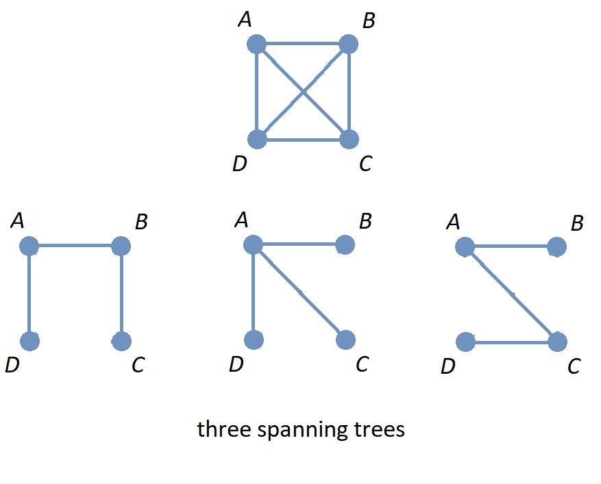
The image shows the graph \(K_{4}\) along with three spanning trees.
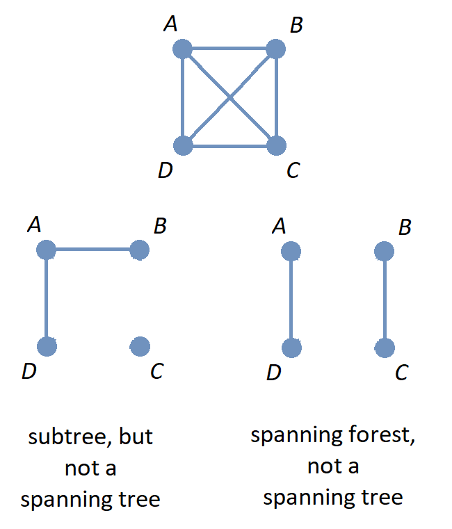
The image shows the graph \(K_{4}\) along with a subgraph that is a subtree that is not a spanning tree, and also a subgraph that is a spanning forest.
Spanning trees are used to solve problems that involve simplifying or optimizing networks. You can learn more about some of the applications of spanning trees at this Wikipedia page.
The following subsection presents one such application.
15.2.1. Minimal-Weight Spanning Trees in Weighted Graphs
In some applications of graphs with weighted edges, you may need to find a spanning tree that has the minimal total weight possible, that is, a spanning tree with sum of edge weights less than or equal to the corresponding sum for any other spanning tree.
Such a spanning tree is referred to as a minimal-weight spanning tree.
Note: Many textbooks and sources use the term minimum length spanning tree because the use of these spanning trees historically arose in problems that involved physical distances between nodes of a network. Other sources use the term minimum spanning tree, abbreviated as MST.
As an example, the image shows a weighted graph along with all three possible spanning trees. The minimal-weight spanning tree, with total weight 6, is drawn on the lower left.
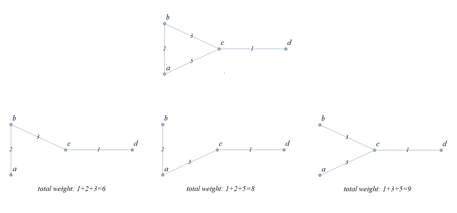
Notice that for the graph in the image, it was both easy and efficient to use “brute force” to look at all of the spanning trees and compute all of the sums of weights for those spanning trees. For weighted graphs that have many more vertices and/or edges, you will need to use a more efficient problem-solving strategy. This textbook discusses one such strategy, Kruskal’s algorithm, in detail.
Kruskal’s Algorithm
Joseph Kruskal published a paper in 1956 that describes an algorithm for constructing “the shortest spanning subtree” of a connected simple graph (Kruskal assumed that the graph has only finitely-many edges, and that each edge has a positive weight which represents the distance between its endpoints.)
-
Task: Given a connected graph \(G = (V,E)\) with weighted edges, construct a spanning tree of \(G\) that has the minimal possible sum of weights.
-
Input: The list \(E\) of all weighted edges of the graph.
-
Steps:
-
Sort the list of edges \(E\) so that each edge \(e_{k}\) in the list has a weight that is less than or equal to the next edge \(e_{k+1}\) in the list.
-
Define the list \(E_{chosen}\) and initialize it as an empty list.
-
Set integer index variable \(i\) to 0.
-
While \(i\) is less than \(|E|,\) the number of edges
-
If it is impossible to form a cycle using edge \(e_{i}\) along with some (or all) of the edges in list \(E_{chosen}\)
-
Append \(e_{i}\) to \(E_{chosen}\)
-
-
Increment \(i\) by 1
-
-
-
Output: The list \(E_{chosen}\) of weighted edges.
Notice that the output list \(E_{chosen}\) was constructed so that its edges cannot be used to form a cycle in the graph \(G.\) Also, since the graph \(G\) is assumed to be connected, every vertex will be the endpoint of at least one edge in \(E_{chosen},\) so that the graph with vertex set \(V\) and edge set \(E_{chosen}\) will be a spanning tree of \(G.\)
Also notice that the condition for the while loop can be changed to “while \(|E_{chosen}| < |V| - 1\)” since a spanning tree must have one fewer edges than vertices.
The image shows a drawing of a simple weighted graph along with all three possible spanning trees.
The minimal-weight spanning tree, with total weight 6, is drawn on the lower left.
Let’s trace through the steps of Kruskal’s algorithm to examine how this minimal-weight spanning tree is constructed. The following table represents the input to the algorithm: A list of all the edges of the graph, along with their corresponding weights.
| Edge | Weight |
|---|---|
{c, d} |
1 |
{a, b} |
2 |
{b, c} |
3 |
{a, c} |
5 |
-
Steps:
-
Sort the list of edges of the graph in order of increasing weight (This has already been done in the table shown.)
-
Set \(E_{chosen}\) to the empty list.
-
Set the index \(i\) to 0.
-
Enter the while loop.
- \(i=0\)
-
\(i\) is less than 4, and it is impossible to form a cycle using \(\{c, d\}\) alone,
so set \(E_{chosen}\) to \([\{c, d\}\)] and set \(i\) to 1. - \(i=1\)
-
\(i\) is less than 4, and it is impossible to form a cycle using \(\{a, b\}\) along with the edge in \(E_{chosen} = [\{c, d\}\)]
so set \(E_{chosen}\) to \([\{c, d\} , \{a, b\}\)] and set \(i\) to 2. - \(i=2\)
-
\(i\) is less than 4, and it is impossible to form a cycle using \(\{b, c\}\) along with the edges in \(E_{chosen} = [\{c, d\} , \{a, b\}\)]
so set \(E_{chosen}\) to \([\{c, d\} , \{a, b\}, \{b, c\}\)] and set \(i\) to 3. - \(i=3\)
-
\(i\) is less than 4, but it is possible to form a cycle using \(\{a, c\}\) along with the edges in \(E_{chosen} = [\{c, d\} , \{a, b\}, \{b, c\}\)]
so make no change to \(E_{chosen}\) and set \(i\) to 4. - \(i=4\)
-
Since \(i\) is not less than 4, exit the while loop.
-
The output is \(E_{chosen} = [\{c, d\} , \{a, b\}, \{b, c\}\)] which is the list of edges used in the spanning tree drawn on the lower left of the image. That is, in at least this one case, the algorithm does construct a minimal-weight spanning tree.
That is, how could you prove that Kruskal’s algorithm must construct a minimal-weight spanning tree for any input graph that is connected and has finitely-many weighted edges?
Here is an exercise for you to try.
Use Kruskal’s algorithm to find the minimal-weight spanning tree for the following graph.
The image shows a graph with vertices representing ten of the busiest airports, by total cargo throughput, in the United States of America. Each vertex is labeled with the International Air Transport Association code for one of the airports, and
each edge represents the route between the two airports at the endpoints.
Image credit: Remixer-created derivative of original work "9-simplex graph.png". The original work has been released into the public domain by its author, Tomruen at English Wikipedia. This applies worldwide.
This table lists each edge with its corresponding weight.
You can download the table as a tab-delimited text file to import the data into a spreadsheet app to sort the list.
You also can view the graph as a map of the routes between the airports at Markus Englund’s Great Circle Map website.
Try to work this out on your own, then confirm that you correctly found the minimal-weight spanning tree by clicking to see the answer below.
Image credit: Remixer-created derivative of original work "9-simplex graph.png". The original work has been released into the public domain by its author, Tomruen at English Wikipedia. This applies worldwide.
The table lists the edges of the minimal-weight spanning tree. + +
A map view of the minimal-weight spanning tree can be seen at the Great Circle Map website.
Other Algorithms for Minimal-Weight Spanning Trees
Among the other algorithms that can be used to find a minimal-weight spanning tree are Borůvka’s algorithm and Prim’s algorithm (also known as the DJP algorithm.) You can learn more about these and other algorithms and their history starting with this section of the Wikipedia page about MSTs, as well as the section Historical Notes from Applied Combinatorics by Keller and Trotter.
In 2002, Pettie and Ramachandran published a paper for an optimal minimum spanning tree algorithm.
15.3. Directed Trees
Recall that a tree is defined to be a connected simple graph that contains no cycles. The edges of a tree are undirected.
However, there are applications where it is useful to think of a tree as having directed edges. For that purpose, a directed tree is defined to be a directed graph whose underlying graph is a tree.
15.3.1. Rooted Trees
In some applications of directed trees, you can view the directed tree as if all paths “flow away” from a single vertex. For these applications, the concept of a rooted tree is useful.
The set of rooted trees can be defined recursively as follows.
| Basis Step |
A single vertex r is a rooted tree. The vertex r is called the root node of this rooted tree. |
| Recursion |
Suppose that you have a nonempty finite set of already-constructed rooted trees
(which will be called “old rooted trees” below)
such that the following propositions are True: |
The image shows the basis step and represents, in part, the results of the first and second uses of the recursion step. In the image, the new root node created at each step is drawn at the top of the rooted tree.
| Notice that the directed edges of rooted trees are drawn without arrows! Computer scientists usually follow this convention: A rooted tree is drawn with the root node at the top, with all the old root nodes of the previously-constructed rooted trees attached in the Recursion step drawn at the same horizontal level beneath the root node. This convention, along with the recursive definition, ensures that the direction of each directed edge is “down,” so an arrow is not needed to determine the direction of edge. |
Notice that if you want to construct just one particular rooted tree, you only need to use the Recursion step finitely-many times. However, at each use of the Recursion step, there is an infinite number of possible rooted trees that can be constructed. Also, to construct all possible rooted trees would require infinitely-many uses of the Recursion step.
Some of the terminology used with rooted trees is borrowed from “family trees,” and other terminology is borrowed from plant science.
-
The new root node \(r\) added in the Recursion step is called the parent of each of the old root nodes, and each of the old root nodes is called a child of \(r.\) The old root nodes collectively are called the children of \(r.\)
-
Two or more nodes with the same parent are called siblings.
-
A node that has one or more children is called an internal node.
-
A node that has no children is called a leaf. A leaf can also be called an external node.
-
The depth of node \(v\) in a rooted tree is the length of the shortest path from the root node \(r\) to the node \(v.\) This is also called the level of the node \(v.\)
-
A level of a rooted tree is the set of all nodes at the same depth. For example, level 1 is the set of all the child nodes of the root node. Level 0 is the set containing only the root node.
-
The height of a rooted tree is the maximum of the depths of all the nodes in the rooted tree.
The next lemma shows that you can construct any rooted tree without using recursion by instead starting with a tree then replacing all the undirected edges by appropriately directed edges.
In summary, the lemma tells you that every rooted tree can be thought of as an adaptation of a tree, where you first select a vertex to be the root node and then replace all the edges of the tree by directed edges that “flow away” from the root node.
15.3.2. Ordered Trees
Notice that in the Recursion step of the definition of rooted tree, the new root node is connected to each of the old root nodes, but since the subtrees' roots are members of a set, the order in which the new root node is connected to the old root nodes is not important. However, in some applications of rooted trees, it is important to note the order in which the new root node is connected to the old root nodes.
For example, in a family tree, you may want to represent a person by the root node of the tree, then represent their offspring by birth order as the child nodes. In this case, the order of the children matters. To do this, you can list the old subtrees as the sequence \(T_{1}, \, \ldots \, T_{n}\) and list the old root nodes as the sequence \(r_{1}, \, \ldots \, r_{n},\) where \(n\) is the number of old subtrees used in the Recursion step.
In this subsection, a recursive definition for ordered trees is presented. This recursive definition takes the order of the indices of the old ordered trees into account when constructing the new ordered tree.
Warning: Many other names for ordered trees appear in various sources, such as ordered rooted tree, rooted plane tree, RP-tree, and decision tree. In fact, some sources even define “rooted tree” to mean what this textbook calls and “ordered tree.”
The set of ordered trees is defined recursively as follows.
| Basis Step |
A single vertex r is an ordered tree. Vertex r is the root node of this ordered tree. |
| Recursion |
Suppose that you have already constructed the ordered trees in the sequence \(T_{1}, \, \ldots \, T_{n}\) where \(n\) is a positive integer and for each positive integer \(i \leq n,\) the root node of \(T_{i}\) is the vertex \(r_{i}.\) |
Ordered trees are usually drawn so that the root node appears at the top of the tree, and for each internal node, the children are drawn in order from left to right.
In summary, an ordered tree can be thought of as a special kind of rooted tree where the children of each internal node are ordered.
15.3.3. Isomorphisms: Rooted Trees and Ordered Trees
As discussed in the Graphs chapter, the definition of isomorphism can be adapted to include one-to-one correspondences between the vertex sets of two graphs that preserve specific features of a graph in addition to the adjacency relationships between vertices. Examples of such features are edge weights, edge directions, vertex colors, or edge colors.
In this subsection, examples are presented to show how the definition of isomorphism can be adapted for rooted trees and ordered trees.
Nonisomorphic Rooted Trees with Isomorphic Underlying Graphs
Here is a question for you: In the image, do the two drawings represent graphs or rooted trees? It’s okay if you are not sure how to answer this question. Since rooted trees are usually drawn with edges that do not use arrows to indicate the direction, the drawings are ambiguous, and you would probably need more context to decide whether the drawings represent two undirected graphs or two rooted trees.
Notice that the interpretation also effects whether the two drawings represent isomorphic objects.
-
Suppose that the drawings are interpreted as undirected graphs. These are isomorphic as undirected graphs, and also isomorphic as trees, since redrawing the graph on the left as the one on the right does not change the adjacency relationships of the vertices.
-
Suppose that the drawings are interpreted as rooted trees. The adjacency relationships are the same, but the direction of the edge with endpoints \(A\) and \(B\) depends on whether \(A\) or \(B\) is chosen as the root node. The underlying graphs with undirected edges are isomorphic, but the rooted trees are not isomorphic.
Nonisomorphic Ordered Trees that are Isomorphic Rooted Trees
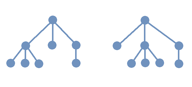
In the image, two rooted trees are shown. The two rooted trees are isomorphic as rooted trees since the order of the children of the root node does not matter. However, these two rooted trees are not isomorphic as ordered trees since the corresponding children are not in the same order in each rooted tree.
It may be helpful to think of each of the two ordered trees as “telling a story” about a family.
-
On the left, a parent has three children, and the oldest child has three children, the middle child has no children, and the youngest child has one child.
-
On the right, a parent has three children, and the oldest child has no children, the middle child has three children, and the youngest child has one child.
In general, ordered trees are isomorphic if and only if they tell the same story about the families, so these two are not isomorphic as ordered trees. On the other hand, they are isomorphic as rooted trees because they tell the same story when the birth order of the children at level 1 is ignored: A parent has three children, of whom one has three children, another one has one child, and yet another one has no children.
15.4. Binary Trees
| As mentioned near the beginning of this chapter, much of the terminology related to trees is not standardized. The definitions in this section use terminology consistent with Handbook of Graph Theory, Second Edition, but information on alternative definitions is also stated. |
For any positive integer \(m,\) an m-ary tree is defined to be
an ordered tree
in which each internal node has at most \(m\) children.
Some sources define m-ary tree to be a rooted tree instead of an ordered tree.
A binary tree is a 2-ary tree, or more simply, an ordered tree in which each internal node has at most two children. In a binary tree, the root node is the parent of at most two subtrees \(T_{1},\) called the left subtree, and \(T_{2},\) called the right subtree. Notice that in the context of binary trees, it is allowable for either or both of the subtrees to be absent (that is, empty).
Some sources allow a binary tree to be “empty,” in the sense that it has no vertices or edges. An “empty binary tree” is not an ordered tree as defined above since it has no root node. However, an empty binary tree is useful in computer science applications. For example, when implementing binary trees as data structures, an empty binary subtree corresponds to by a null pointer (or null reference); a leaf node of a binary tree can be recognized as a node whose left child and right child pointers/references are both null.
A complete binary tree is a binary tree in which every internal node has exactly 2 children and all leaves are at the same level.
Some sources use either “perfect binary tree” or “full binary trees” to describe this type of binary tree and use the phrase “complete binary tree” to describe something else.
A binary tree is called balanced if for every vertex \(v,\) the number of vertices in the left subtree of \(v\) and the number of vertices in the right subtree of \(v\) differ by at most one.
Some sources define a binary tree of height \(h\) to be balanced if each leaf is at either level \(h\) or level \(h − 1.\)
15.4.1. Tree Traversal Algorithms for Binary Trees
In many applications of binary trees, it is necessary to visit every node. The process of visiting every node is called tree traversal. In this subsection, you will learn about three commonly-used algorithms for tree traversal.
The three traversal algorithms can be described recursively as follows.
-
Preorder traversal: First, visit the root node. Secondly, visit each node in the root node’s left subtree using preorder traversal. Finally, visit each node in the root node’s right subtree using preorder traversal.
-
Inorder traversal: First, visit each node in the root node’s left subtree using inorder traversal. Secondly, visit the root node. Finally, visit each node in the root node’s right subtree using preorder traversal.
-
Postorder traversal: First, visit each node in the root node’s left subtree using postorder traversal. Secondly, visit each node in the root node’s right subtree using postorder traversal. Finally, visit the root node.
For each of these three traversal algorithms, the Base Step for the recursion
is applied to
a binary tree that has only one node
(a root node that has empty left and right subtrees),
and
you visit just that one node.
Some sources use hyphens in the written names of these traversal algorithms, so list them as pre-order, in-order, and post-order traversal.
The image displays the same binary tree with its nodes being “counted off” using each of these three traversal algorithms.
You may find the interactive demonstration at this Wikipedia page useful to understanding these three traversal algorithms.
15.4.2. Binary Search Trees
Define a key to be an element of a set that has a total ordering. For example, keys could be integers ordered using the usual \(\leq\) relation. As another example, keys could be strings ordered alphabetically. In general, keys could be any type of data that can be totally ordered.
A binary search tree (BST) is a binary tree where each vertex is assigned a key in such a way that that if key \(k\) is assigned to vertex \(v\) then both of the following are True.
-
the key \(k\) is greater than each key assigned to a vertex in the left subtree of \(v,\) and
-
the key \(k\) is less than each key assigned to a vertex in the right subtree of \(v.\)
If you are given a list (or an array) of keys, a binary search tree can be used to sort the keys and then quickly search for a key. An advantage of binary search trees is that it is much easier and faster to maintain the sort order if you need to insert new keys than it would be to insert the same keys into a sorted list (or an array) of keys.
First, let’s construct a binary search tree from the list of keys \( \left[ 17, 3, 5, 31, 2 \right .\)]
-
The first key in the list, \(17,\) is assigned to the root node.
-
The next key, \(3,\) is less than the key \(17\) at the root node, so \(3\) is assigned to the left child of the root node.
-
The next key, \(5,\) is less than the key \(17\) at the root node, so \(5\) must be assigned to some node in the left subtree.
-
Since \(5\) is greater than the key \(3\) at the left subtree’s root, \(5\) is assigned to the right child of the left subtree’s root.
-
-
The next key, \(31,\) is greater than the key \(17\) at the root node, so \(31\) is assigned to the right child of the root node.
-
The last key, \(2,\) is less than the key \(17\) at the root node, so \(2\) must be assigned to some node in the left subtree.
-
Since \(2\) is greater than \(3,\) \(2\) is assigned to the left child of of the left subtree’s root.
-
The following animation illustrates the construction of this binary search tree.

Now, let’s search for some keys. If a key is not already present, it will be inserted in the correct position.
Consider the key \(5.\)
-
\(5\) is less than the key at the root node, which is \(17.\) If \(5\) is in this BST, it must be in the left subtree, so continue searching from there.
-
\(5\) is greater than the key at the left subtree’s root node, which is \(3.\) If \(5\) is in this BST, it must be in the right subtree of this node, so continue searching from there.
-
\(5\) is equal to the key at the subtree’s root node, so we have found this key!
Now consider the key \(19\) which was not included in the original list.
-
\(19\) is greater than the key at the root node, which is \(17.\) If \(19\) is in this BST, it must be in the right subtree, so continue searching from there.
-
\(19\) is less than the key at the right subtree’s root node, which is \(31.\) If \(19\) is in this BST, it must be in the left subtree of this node, so continue searching from there.
-
This subtree is empty, so insert a new root node for this subtree and assign the key \(19\) to this new node.
The following image shows the modified BST with the new key \(19\) inserted in the correct position.
Locate the correct position of the new node when the key \(11\) is inserted in the previously modified BST.
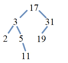
Constructing a binary search trees from a list can serve two purposes. First, as shown in the preceding example, it is quicker to search for a key in the binary search tree because, in the best case scenario when the tree is balanced, the number of keys is halved with each iteration of the search. Secondly, the original list can be sorted by performing an inorder traversal of the binary search tree.
Consider the binary search tree with integer keys that was the solution in the “You Try” section of the previous example.

List the keys of the binary search tree using each of preorder, inorder, and postorder traversal to visit all nodes of the binary search tree.
Inorder: \( \left[ 2, 3, 5, 11, 17, 19, 31 \right .\)]
Preorder: \( \left[ 2, 11, 5, 3, 19, 31, 17 \right .\)]
Here is another exercise for you to try.
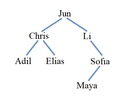
15.4.3. Expression Trees and Polish Notation
In the 1920’s, the Polish logician Jan Łukasiewicz created a notational format for writing logical well-formed formulas that does not use any parentheses: Instead of writing logical operator symbols (like \(\land\) and \(\lor\)) between two previously-constructed wffs, Łukasiewicz placed operator symbols in front of those wffs, which makes the use of parentheses completely unnecessary! Today, notation that is based on Łukasiewicz’s original notation is called either Polish notation or prefix notation and is applied to both arithmetic/algebraic formulas and logical formulas.
There is also the Reverse Polish notation, also called postfix notation, where the operator symbol is placed after its operands. The “usual” notation where the operator symbol is placed between the two operands is called infix notation.
You can use binary trees and tree traversal to make it easier to switch between these three notations. Define an expression tree to be a binary tree where each leaf is labeled by either a numeral or a variable symbol, and where each internal node is labeled by an operator symbol. The expression tree for the infix notation \(3 \cdot x - 5\) is shown. Notice that in the expression tree for \(3 \cdot x - 5,\) the root node corresponds to the “last” operation you would perform and the subtrees correspond to the previously-constructed expressions \(3 \cdot x\) and \(5.\) Also notice that, in the earlier example, the order of the symbols for the infix expression corresponds to the inorder traversal of the expression tree. It is an exercise for you to confirm that the order of the symbols in the Polish notation expression corresponds to the preorder traversal of the expression tree, and that the Reverse Polish notation expression corresponds to the postorder traversal of the expression tree.
Consider the arithmetic expression. \[ 5 + 7 \times - 3 - 8 \div 2 \] Recall that it is not correct to evaluate this left-to-right; instead you need to use the order of operations, which is equivalent to evaluating the following expression that results after inserting parentheses. \[ (5 + (7 \times (- 3))) - (8 \div 2) \] From this second expression, you can see that the expression tree will have the minus sign at the root and subtrees that represent \((5 + (7 \times (- 3)))\) and \((8 \div 2).\) Continuing recursively, the subtree for \((5 + (7 \times (- 3)))\) will have the plus sign at its root and subtrees that represent \(5\) and \((7 \times (- 3)),\) and the subtree for \((8 \div 2)\) will have the division sign at its root node and subtrees that represent \(8\) and \(2.\) Continue recursively until all symbols have been placed at a node.
The image displays a drawing of the expression tree for \((5 + (7 \times (- 3))) - (8 \div 2)\). Notice that the negative sign labels a node with only one child, which is treated as the left child (but as the right child for inorder traversal.)
Next, you can use each of the traversal methods to create the Polish (prefix), infix, and Reverse Polish (postfix) expressions.
\(\text{prefix: } \ - \, + \, 5 \, \times \, 7 \, - \, 3 \, \div \, 8 \; 2 \)
\(\text{infix: } \ 5 \, + \, 7 \, \times \, - \, 3 \, - \, 8 \, \div \, 2 \)
\(\text{postfix:} \ 5 \, 7 \, 3 \, - \, \times \, + \, 8 \; 2 \, \div \, - \)
You can see another example of how to construct expression trees, using Reverse Polish notation and a stack, at this Wikipedia page.
15.4.4. Isomorphisms: Binary Trees
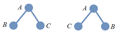
In the image, two binary trees are shown. As binary trees are ordered trees, it should be clear that these cannot be isomorphic as binary trees because the order of the left and right children of the root node in the two trees are different.
15.5. Additional Topics To Be Added Later
-
Algorithms for Depth- and breadth-first traversals
16. Appendix: On-Demand Math Resources
NOTICE: If you are NOT enrolled in the CSC 230 course that I teach at SFSU, you probably are looking for the “public version” of the book, which I only update between semesters. The version you are looking at now is the “CSC230 version” of the book, which I will be updating throughout the semester.
This chapter was last updated on August 25, 2024.
This appendix discusses material that you have likely seen before but may need some review.
16.1. Linear Functions And Their Equations
A linear function is one that has a constant rate of change.
\begin{array}{|l|c|c|c|c|c|} & x & 1 & 2 & 3 & 4 & 5 \\ \hline \\ & y & 1 & 3 & 5 & 7 & 9 \end{array}
The table above displays a function with independent variable \(x\) and dependent variable \(y\).
Notice that the value of \(y\) increases by \(2\) for each increase in \(x\) by \(1\). The rate of change of this function is \(2\); this corresponds to the slope \(m\) of the continuous line that passes through the points with \(xy\)-coordinates given in the table.
The vertical intercept \(b\) (in this case, the y-_intercept) is the \(y\)-value that corresponds to \(x = 0\), that is, \((0,\,b)\) is on the same continuous line as the points represented in the table. In this example, \(0\) is not a value of \(x\), but we can still find the vertical intercept by _subtracting \(1\) from the smallest \(x\)-value and subtracting \(2\) from the corresponding \(y\)-value , which tells us that the point \((0,\,-1)\) lies on the same continuous line as the points represented in the table.
The equation of the linear function determined by the points in the table is \(y = 2 \cdot x + (-1)\), which can be written more simply as \(y = 2x - 1\). This also is the equation of the continuous line that passes through the points with \(xy\)-coordinates given in the table, but the linear function can be restricted to a smaller domain as needed by the context where it is being used, for example, we may only need to use inputs \(x\) from the set of positive integers or possibly just the set \(\{ 1,\,2,\,3,\,4,\,5 \}\).
16.2. Arithmetic Sequences
An arithmetic sequence or arithmetic progression is a sequence of numbers \(a_{0}, \, a_{1}, \, a_{2}, \, \ldots\) such that there is a constant \(d\) so that \[ a_{i+1}-a_{i} = d \text{ for all } i \in \mathbb{N}\] The constant \(d\) is called the common difference of the sequence. The sequence can be infinite, defined for every \(i \in \mathbb{N},\) or finite, defined only for \(i \in \mathbb{N}\) less than some greatest index \(n\).
As an example, the sequence \(1, 4, 7, 10, 13, 16\) is a finite arithmetic sequence with common difference 3 and index set \(\{ 0, 1, 2, 3, 4, 5 \}.\) We can extend that sequence to an infinite arithmetic sequence \(1, 4, 7, 10, 13, 16, \ldots\) using a recursive definition \[a_{0} = 1, \text{ and } a_{i+1} = a_{i} + 3 \text{ for integer } \in \mathbb{N} \]
Notice that there is also a nonrecursive definition for this sequence: Since the difference between two consecutive terms of the sequence is always \(d\) the points \((i, \, a_{i})\) must lie on a line in the xy-plane. The slope of this line is \(d\) and the y-intercept of the line is the initial value \(a_{0},\) so the arithmetic sequence can also be described as \[ a_{i}= d \cdot i + a_{0} \text{ for all } i \in \mathbb{N}\]
For the example \(1, 4, 7, 10, 13, 16, \ldots\), the nonrecursive definition is \[a_{i} = 3i + 1 \text{ for all } i \in \mathbb{N}\]
16.3. Geometric Sequences
A geometric sequence or geometric progression is a sequence of numbers \(a_{0}, \, a_{1}, \, a_{2}, \, \ldots\) such that there is a constant \(r\) so that \[ a_{i+1} = r \cdot a_{i} \text{ for all } i \in \mathbb{N}\] The constant \(r\) is called the common ratio of the sequence. The sequence can be infinite, defined for every \(i \in \mathbb{N},\) or finite, defined only for \(i \in \mathbb{N}\) less than some greatest index \(n\).
As an example, the sequence \(5, 10, 20, 40, 80\) is a finite geometric sequence with common ratio 2 and index set \(\{ 0, 1, 2, 3, 4 \}.\) We can extend that sequence to an infinite geometric sequence \(5, 10, 20, 40, 80, \ldots\) using a recursive definition \[a_{0} = 5, \text{ and } a_{i+1} = a_{i} \cdot 2 \text{ for integer } i \in \mathbb{N} \]
There is also a nonrecursive definition for this sequence: Since the ratio between a term and its predecessor in the sequence is always \(r\) the points \((i, \, a_{i})\) must lie on the graph of an exponential function in the xy-plane. The y-intercept of the graph is the initial value \(a_{0},\) so the geometric sequence can be described as \[ a_{i} = a_{0} \cdot r^{i} \text{ for all } i \in \mathbb{N}\]
For the example \(5, 10, 20, 40, 80, \ldots\), the nonrecursive definition is \[a_{i} = 5 \cdot 2^{i} \text{ for all } i \in \mathbb{N}\]
MORE TO COME!
17. Appendix: Library of Functions
NOTICE: If you are NOT enrolled in the CSC 230 course that I teach at SFSU, you probably are looking for the “public version” of the book, which I only update between semesters. The version you are looking at now is the “CSC230 version” of the book, which I will be updating throughout the semester.
This chapter was last updated on August 24, 2025.
repaired some typos
Recall that for any function,
-
the domain is the given set of input values for the function,
-
the codomain is a given set that contains all possible output values (but may contain other values that are not outputs, too), and
-
the range is the set that contains only the output values of the function.
Functions can in many cases be visualized graphically, for example when mapping from the real line, \(\mathbb{R}\) to the real line, such maps are viewed on a Cartesian plane.
17.1. Polynomial Functions
A polynomial is an algebraic expression of the form \(a_{n}x^{n} + a_{n-1}x^{n-1} + \ldots + a_{1}x^{1} + a_{0}\), that is, \(\sum\limits_{i=0}^{n}a_{i}x^{i}\), where n is a natural number, x is a variable, and \(a_{n}, a_{n-1}, \ldots, a_{1}, a_{0}\) are real numbers. Examples of such expressions are
-
7, a constant,
-
\(2x + 7\), a linear polynomial,
-
\(3x^{2} + 2x + 7\), a quadratic polynomial.
A polynomial can be evaluated by substituting a number for each occurence of x. For example, if we substitute \(-1\) for x in each of the three polynomials above, we get
-
7 evaluated at \(x = -1\) is 7,
-
\(2x + 7\) evaluated at \(x = -1\) is \(2 \cdot (-1) + 7 = 5\),
-
\(3x^{2} + 2x + 7\) evaluated at \(x = -1\) is \(3 \cdot (-1)^{2} + 2 \cdot (-1) + 7 = 8.\)
In this way, every polynomial can be used to define a corresponding polynomial function with domain \(\mathbb{R}\) and codomain \(\mathbb{R}.\)
17.1.1. Quadratic Function
The function \(f(x) =x^2\), denotes the association \((a,b) =(x, x^2)\) with \(f : \mathbb{R} \rightarrow \mathbb{R}\). We notice that the range is the set of real numbers \([0, \infty)= \mathbb{R}^{+}\). The function is not invertible, since it is not injective. For example, we have both \(f(-3) =9\) and \(f(3)=9\). With \(f : \mathbb{Z} \rightarrow \mathbb{Z}\) notice that the range is now \(\mathbb{N}\)
\begin{array}{lccccccccccc} & x & -5 & -4 & -3 & -2 & -1 & 0 & 1 & 2 & 3 & 4 & 5 \\ & x^2 & 25 & 16 & 9 & 4 & 1 & 0 & 1 & 4 & 9 & 16 & 25 \end{array}
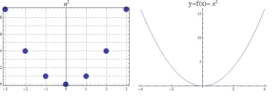
17.1.2. The Cubic function
The function \(f(x) =x^3\), denotes the association \((a,b) =(x, x^3)\) with \(f : \mathbb{R} \rightarrow \mathbb{R}\). Also, we notice that the range is the set of all real numbers \((- \infty , \infty)=\mathbb{R}\). The function is bijective and so invertible. With \(f : \mathbb{Z} \rightarrow \mathbb{Z}\), notice that the range, in addition to domain, is also \(\mathbb{Z}\)
\begin{array}{llcccccccccl} & x & -5 & -4 & -3 & -2 & -1 & 0 & 1 & 2 & 3 & 4 & 5 \\ & x^3 & -125 & -64 & -27 & -8 & -1 & 0 & 1 & 8 & 27 & 64 & 125 \end{array}
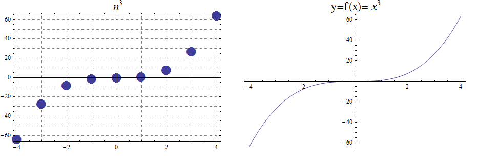
17.1.3. The Square Root and Cube Root Functions
For the purposes of completeness and for comparing how fast functions \(f(x)\) grow for large x, we present the inverse of the functions \(f(x)= x^2\) and \(f(x)= x^3\), when \(f(x):\mathbb{R}+→\mathbb{R}+\). Respectively, the functions\( f(x)=\sqrt{x}\) and \(f(x)= \) \$root(3)(x)\$.
\begin{array}{lcccccccccclll} & x & 0 & 1 & 4 & 9 & 16 & 25 & 36 & 49 & 64 & 81 & 100 & 121 & 144 \\ & \sqrt{x} & 0 & 1 & 2 & 3 & 4 & 5 & 6 & 7 & 8 & 9 & 10 & 11 & 12 \end{array}
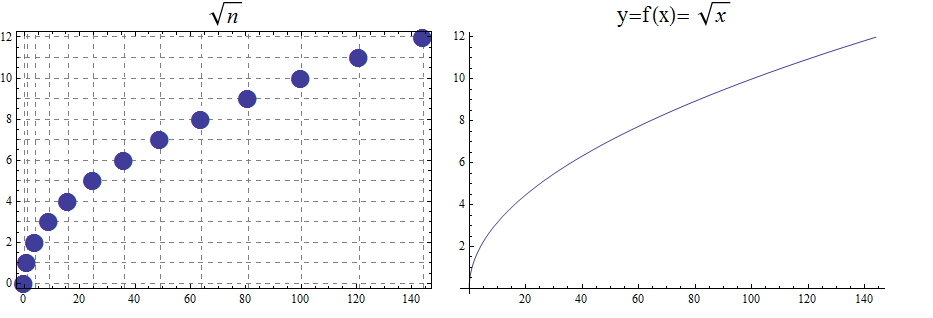
\begin{array}{lcccccl} & x & 0 & 1 & 8 & 27 & 64 & 125 \\ & \sqrt[3]{x} & 0 & 1 & 2 & 3 & 4 & 5 \end{array}
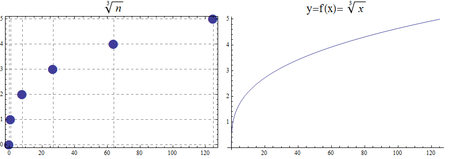
17.2. Exponential and Logarithmic Functions
We begin by summarizing important properties of exponentials.
17.2.1. Exponential Functions
Exponential functions are of the form \(f\left(x\right)=b^x\), where \(b\) is the base and the variable \(x\) is in the exponent. The base \(b>0\) and \(b ≠ 1\). Properties of exponential functions come from properties of exponents. When the base \(b\) is greater than 1 the exponential function is increasing exponentially, as in the case \(f(x) = 2^x\).
\begin{array}{llcccccccccl} & x & -5 & -4 & -3 & -2 & -1 & 0 & 1 & 2 & 3 & 4 & 5 \\ & 2^x & \frac{1}{32} & \frac{1}{16} & \frac{1}{8} & \frac{1}{4} & \frac{1}{2} & 1 & 2 & 4 & 8 & 16 & 32 \end{array}
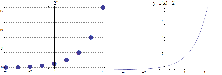
When the base \(b\) is less than 1 the exponential function is decreasing exponentially, as in the case \(f(x) = \left(\frac{1}{3}\right) ^x\).
\begin{array}{llcccccccccl} & x & -5 & -4 & -3 & -2 & -1 & 0 & 1 & 2 & 3 & 4 & 5 \\ & (\frac{1}{3})^x & 243 & 81 & 27 & 9 & 3 & 1 & \frac{1}{3} & \frac{1}{9} & \frac{1}{27} & \frac{1}{81} & \frac{1}{243} \end{array}
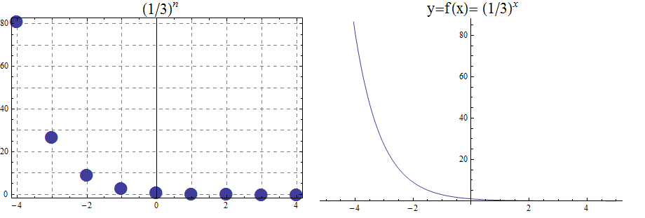
17.2.2. Logarithmic Functions
Logarithmic functions are the inverse functions corresponding to exponential functions and are used to solve exponential equations. For example, \(y=2^x\) is solved for \(x\) by inverting \(x=\log_2{y}\). Properties of logarithms follow from this relationship between exponentials and logarithms and properties of the exponentials.
We summarize three important properties of logarithms.
All other properties of logarithmic functions come from properties relating the logarithm as the inverse of the exponential and the equivalence of the logarithm \(a =\log_b m\) with \(b^a=m\).
When the base \(b\) is greater than 1, the logarithm function is increasing, as in the case \(f(x) = \log_2 x\).
\begin{array}{llllllcccccc} & x & \frac{1}{32} & \frac{1}{16} & \frac{1}{8} & \frac{1}{4} & \frac{1}{2} & 1 & 2 & 4 & 8 & 16 & 32 \\ & log_2 x & -5 & -4 & -3 & -2 & -1 & 0 & 1 & 2 & 3 & 4 & 5 \end{array}
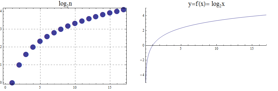
When the base \(b\) is less than 1, the logarithm function is decreasing exponentially, as in the case \(f(x) = \log_{\frac{1}{3}} \ x\).
\begin{array}{llllllcccccl} & x & \frac{1}{243} & \frac{1}{81} & \frac{1}{27} & \frac{1}{9} & \frac{1}{3} & 1 & 3 & 9 & 27 & 81 & 243 \\ & \log_{\frac{1}{3}} x & 5 & 4 & 3 & 2 & 1 & 0 & -1 & -2 & -3 & -4 & -5 \end{array}
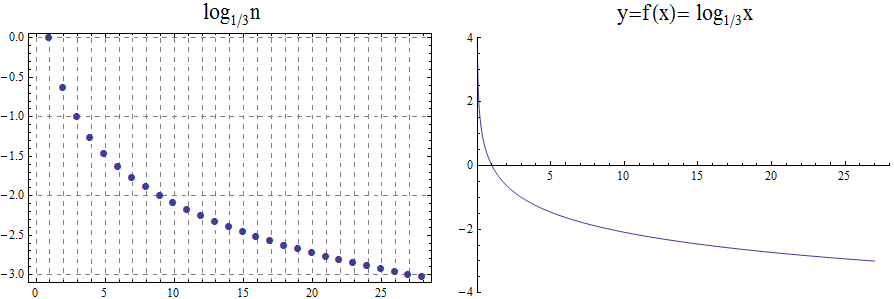
17.3. The Floor and Ceiling Functions
The floor and ceiling functions round a real number input to an integer.
-
The floor of x, written as \(\lfloor x \rfloor,\) is the greatest integer that is less than or equal to x. In older textbooks you may see this function named as the greatest integer function and denoted by \([ x ] .\) For example, \(\lfloor -1.5 \rfloor = -2\).
-
The ceiling of x, written as \(\lceil x \rceil,\) is the least integer that is greater than or equal to x. For example, \(\lceil -1.5 \rceil = -1\).
On a number line, the floor of x and the ceiling of x are the consecutive integers such that \(\lfloor x \rfloor \leq x \leq \lceil x \rceil\).
The floor and ceiling functions are step functions: In the plane, their plots look like they are made of horizontal steps.
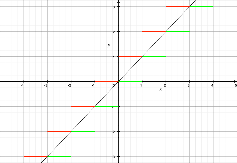
Note that the plot of the floor function, shown in green, is always at the same height or below the graph of the line \(y = x\), and that the plot of the ceiling function, shown in red, is always at the same height or above the graph of the line \(y = x.\)
17.4. Other Functions
MORE TO COME!!
18. Appendix: An Introduction to Python
NOTICE: If you are NOT enrolled in the CSC 230 course that I teach at SFSU, you probably are looking for the “public version” of the book, which I only update between semesters. The version you are looking at now is the “CSC230 version” of the book, which I will be updating throughout the semester.
18.1. Programming Basics
Computers are programmable machines that process information by manipulating data. As the data can represent any real world information, and programs can be readily changed, computers are capable of solving many kinds of problems.
18.1.1. Programming Languages and Environments
There are many different programming languages for programmers to choose from. Each language has its own advantages and disadvantages, and new languages gain popularity while older ones slowly lose ground. In this book, we use the Python 3 programming language. It is popular in both academia and industry, and was designed with education in mind.
18.1.2. PythonTutor
PythonTutor is an environment for creating very short and simple Python programs and visualizing their execution. This enables beginners to visually see the data as it gets manipulated by the instructions.
18.1.3. Comments
Program files can contain source code and comments. Comments are not instructions for the computer to follow, but instead notes for programmers to read. Comments in Python start with a pound sign (#). Anything following the pound sign that is on the same line as the pound sign will not be executed. Often, at the very beginning of a program, comments are used to indicate the author and other information. Comments are also used to explain tricky sections of code or disable code from executing.
# This line is not Python code, it is a comment.

score = 9001 # over 9000!!!

# The next line of code is disabled because is starts with a #.
# score = 8000
18.2. Data Types
Programming is all about information processing. Information is categorized by data types. Four basic data types we will be considering are int, float, bool, and str. Int consists of integers, which are whole numbers written without a decimal point. This includes positive and negative whole numbers as well as zero. Float consists of floating-point numbers, which are numbers that are written with a decimal point. Bool consists of Boolean values (named after the mathematician George Boole). The only Boolean values are True and False. Str consists of strings, which are sequences of text characters including punctuation, symbols, and whitespace. Every value in Python has a corresponding data type. The table below shows examples of ints, floats, and strings.
| Data Type | Example Values |
|---|---|
int |
2, -2, 0, 834529 |
float |
3.14, -2.3333, 7.0 |
bool |
True, False |
str |
"Hello World!", 'Coconut', "0", '4 + 6' |
|
Strings and Quotation Marks
Strings are always surrounded by quotation marks. Python allows either single (') or double (") quotation marks for single line strings. Python also allows triple quotation marks (either ''' or """) for a string that spans multiple lines. |
18.3. Variables
Variables are (virtual) boxes that store values for reuse later. A variable has a name and a current value. Each variable can only hold one value at a time. Variables are assigned a value using the single equal sign (=). As Python executes one line at a time, variables come into existence on the line where they are first assigned. Each variable only stores the most recent value assigned to it.
|
Variable Names
Variables can have complex names like player1_score. In general, never start a variable name with a number and never use spaces in variable names. |
18.4. Operators and Expressions
|
Expression Evaluation
When Python encounters a line with an expression, it always evaluates the expression first. Consider the following line of code: Python first calculates the value of the expression to the right of the equal sign by using the standard order of operations starting inside the parentheses. The value given by the above expression is calculated to be equal to 14. Then, Python creates the variable x and assigns the value 14 to this variable. The variable only stores the calculated value, not the entire expression that generated that value. |
18.5. Strings and Printing
Besides creating and storing values in variables, we can also output text on a screen by calling the print() function.
18.6. If Statements
A block of code is a collection of lines of code that are either all executed (in sequential order) or all skipped. Blocks always start with a colon (:) on the previous line and require every line in the block to be indented the same amount using tabs or spaces. One way in which Python can execute or skip over a block involves using an if command and a Boolean expression. If the expression is true, then the block executes. Othewise, the block is skipped.
When you want to force exactly 1 of 2 blocks to execute (as opposed to just skipping a block), you can use the else command in addition to the if command. If the expression following the if command is true, then the first block executes. Otherwise, the second block executes.
In order to force exactly 1 of more than 2 blocks to execute, you can use the elif command in addition to the if and else commands. Each elif command must be followed by a Boolean expression. When using if and elif commands, each expression is checked in sequential order, and the block following the first true expression executes. If none of the expressions are true, the block following the else command is executed.
18.7. While Statements
Python can execute a block repeatedly using a while statement and a Boolean expression. The block repeats until the Boolean expression is false.
| The += operator increases the value of the variable written to the left of the operator by the value written to the right of the operator. |
18.8. Lists and Loops
When you need to consider many values at once, use a list.
When you want to consider every value in a list, use a for loop.
| The range() function returns a sequence of numbers. The sequence starts at the value given by the first argument, increments by 1, and ends at one less than the value given by the second argument. For example, range(2,5) returns 2,3,4. If only one argument is given, that argument is considered the second argument and the first argument is set to 0 by default. For example, range(4) returns 0,1,2,3. |
18.9. List Appending and Slicing
We can append to lists with the concatenation operator (+). We can also slice a list using the bracket notation and two indices separated by a colon (:). The first index specifies the starting point of the slice while the second index specifies the stopping point of the slice + 1.
18.10. Lists versus Arrays
Python has both lists and arrays. Lists are convenient because the items in the list can be of different data types, but all items in an array must have the same data type. Arrays are more efficient because the items are stored in the array, but a list stores only a reference (or pointer) to the actual item. For the purposes of the MKD Remix, lists are preferred, but be aware that in some cases an array may be a better choice than a list. You can read more about arrays here.
18.11. Defining Custom Functions
In the examples above we have called several functions like print() and len(). You can define your own functions using def. A function definition includes zero or more parameter variables. The values of those parameter variables are referred to as the arguments of the function.
18.12. Exercises
-
Given the following Python code, what is the value and data type of each variable?
a = 6 + 8 large = a // 4 b = 22 // 3 c = 22 % 3 d = False or True e = True and False sheep = (True or (b > 10)) -
Given the following Python code, determine the printed output.
print("Hello World!") a = "The answer is" b = 6 * 7 print(a, b) print(False, "Hobbit", 1, "Ring") -
For the following code, determine the value of the variable letter when the score is 92, 84 and 59.
score = #an interger between 0 and 100 if score >= 90: letter = 'A' elif score >= 80: letter = 'B' elif score >= 70: letter = 'C' elif score >= 60: letter = 'D' else: letter = 'F' -
For the following code, determine the value of the variable ans for each case given below.
if outside == False: if (n >= 2 and n <= 20): return ans = True else: return ans = False else: if (n <= 2 or n >= 20): return ans = True else: return ans = False-
n = 3, outside = False
-
n = 15, outside = False
-
n = 15, outside = True
-
n = 12, outside = True
-
-
What will this code print out?
while count > 0: print("Welcome") count -= 1 -
Write Python code to satisfy the following conditions. Then test your code on the values of the variables given.
-
Given an int n, return the absolute diffrence between n and 10, except return triple the absolute dfference if n is over 10. It should return 1 when n=9. It should return 33 when n=21. What will the code return when n=7 or n=35?
-
We have a loud talking robot. The "hour" parameter is the current hour time in the range 0 to 23. We are in trouble if the robot is talking and the hour is before 6 or after 21. Return True if we are in trouble. It should return True when the robot is talking and the hour is 8. It should return False when the robot is not talking and the hour is 8. What does it return if the robot is talking and the hour is 9?
-
-
What will the following code print out?
numbers = [1, 3, 5, 7, 10] sq = 0 for val in numbers: sq = val * val print(sq) -
What will the following code print out?
for i in range(1, 20, 2): print(i) -
Use the following definition of the function front3() to find the output of the program for the list [1, 3, 5, 7].
def front3(nums): i = 0 while (i < len(nums) and i < 5): if nums[i] == 3: return True i += 1 return False -
Write a function that takes, as input, two lists of integers, a and b, both of length 3, and returns, as output, a new list of length 2 containing the last elements of a and b. For example, if a = [1, 2, 3] and b = [10, 20, 30], then the function should return the list [3, 30].
19. Appendix: Python Syntax Examples
NOTICE: If you are NOT enrolled in the CSC 230 course that I teach at SFSU, you probably are looking for the “public version” of the book, which I only update between semesters. The version you are looking at now is the “CSC230 version” of the book, which I will be updating throughout the semester.
1
2
3
4
5
6
7
8
9
10
11
12
13
14
15
16
17
18
19
20
21
22
23
24
25
26
27
28
29
30
31
32
33
34
35
36
37
38
39
40
41
42
43
44
45
46
47
48
49
50
51
52
53
54
55
56
57
58
59
60
61
62
63
64
65
66
67
68
69
70 # the '#' character makes a COMMENT separating Python from English
x = 3 # create the VARIABLE with NAME x and STORE INT VALUE 3
Sebastien_Score = 9001 # variable names can be long, but no spaces!
y = 1.0 * 3 # y stores EXPRESSION's RETURN FLOAT value 3.0
z = "Hi There!" # z stores a STRING value
w = False # w stores a BOOLEAN value
v = [3, 30, "Hello World"] # v stores a LIST of values
print(z) # print function displays output ("Hi There!")
# Maths
a = 3
b = 3.0 # b stores 3.0 (float values are decimal approximations)
c = 7 // 2 # c stores 3 (int division always gives ints)
d = 7 % 2 # d stores 1 (Mod or Remainder of the division)
a = 5 # change the value of a to 5
a += 1 # INCREMENT the value of a by 1 (to 6)
# Boolean Operators
a = (3 > 2) # a stores True because 3 is greater than 2
a = (2 >= 2) # a stores True because 2 is greater than or equal to 2
a = (3 < 2) # a stores False because 3 is not less than 2
a = (2 <= 2) # a stores True because 2 is less than or equal to 2
a = (3 != 2) # a stores True because 3 is not equal to 2
a = (3 == 3) # a stores True because 3 is equal to 3
a = (True and False) # a stores False, AND returns True only when both sides are True
a = (True or False) # a stores True, OR returns True if at least 1 side is True
a = (not False) # a stores True, NOT returns opposite
# BLOCKS are sections of any code chunked together with INDENTATION
# BLOCKS start with a ':' and continue with each INDENTED line
x = 7
if x > 8: # if CONDITION is True, then execute block, otherwise skip block.
print("Hello") # since x stores 7, this will skip
print("I Am Sam.") # since x stores 7, this will skip
elif x > 2: # elif condition is True AND previous if was False, execute block
print("Hi") # since x stores 7, this will execute
print("I am Sally.") # since x stores 7, this will execute
else: # if all previous conditions are False, executer block.
print("Yo") # since x stores 7, this will skip
print("I'm Bob.") # since x stores 7, this will skip
while x > 3: # repeat a block until condition becomes False
print("Apples")
x += -1
# Lists store multiple values
a = [10, 30, 20, 90] # create a new list
x = len(a) # x stores 4 (the length)
b = a[0] # INDEX into the list, 0 is first value, b stores 10
c = a[3] # c stores 90
d = a[-1] # -1 is last value, d stores 90
e = a[1:3] # slice a from index 1 up to index 3, e stores [30, 20]
a[1] = 50 # modify the second element in the list, a is now [10, 50, 20, 90]
f = a + [5, 15] # f stores [10, 50, 20, 90, 5, 15], CONCATENATION not addition
g = range(0, 4) # range function returns list 0 up to 4, g stores [0, 1, 2, 3]
# For Loops
for c in "Elephant!": # repeat block with c storing each character 1 at a time
print(c) # prints one letter per line
for x in [10, 30, 20]:
print(x) # prints one number per line
# Custom Functions
def myfunc(a, b): # DEFINES a new function that takes 2 INPUT PARAMETER values
c = 2 * a + b # executes only when function is called
return c # RETURNS a value back to the calling code
x = myfunc(10, 5) # Calls the myfunc() function, x stores return value 25
y = myfunc(1, 3) # Calls the myfunc() function, x stores return value 5
20. Appendix: For Instructors
CAUTION - CHAPTER UNDER CONSTRUCTION!
NOTICE: If you are NOT enrolled in the CSC 230 course that I teach at SFSU, you probably are looking for the “public version” of the book, which I only update between semesters. The version you are looking at now is the “CSC230 version” of the book, which I will be updating throughout the semester.
This chapter was last updated on August 24, 2025.
made minor wording changes
In this appendix, the remixer shares some ideas that other instructors may find useful.
20.1. Incorporating Lessons from the Discrete Mathematics Project
Here is how I, the remixer, have tried to use the “team-worthy” activity-based lesson materials developed by the Discrete Mathematics Project (DMP) in the course that I teach using the Remix.
It appears that one of the purposes of these lessons is to have each student play one specific role (either Documenter, Reporter, Facilitator, or Questioner) for their team during each lesson. The aim is to give students the experience of being assigned such a role, which may happen in their professional lives.
The order of the lessons in the list below reflects how the remixer has used them throughout a one-semester course.
| Introduction to Teamworthy Tasks - Counting (DMP Lesson 1) |
This lesson involves counting arguments and seems to have been designed as an accessible entry point for all students. |
| Handshake Lemma (DMP Lesson 3) |
This lesson can be used to introduce the concept of conjecture, lay the groundwork for proof, and provides a nonarithmetic/nonalgebraic example for proof by mathematical induction that is referred to later when mathematical induction is formally introduced. The graph theory content needed by students is minimal and can be learned just-in-time, so this lesson can be used very early in the course. NOTE: It may be important to mention to students that this activity does not involve literally shaking the hands of other people. A possible extension to this could be to use directed edges. Also, using this lesson as the first one in a semester may have an advantage over the counting problems included in the Introduction to Teamworthy Tasks lesson: The graph theory content is likely to be unfamiliar to most students so that team members may be more likely to adhere to their specific team roles. |
| Logic & Inference (DMP Lesson 5) |
This lesson focuses on using rules of inference to make a valid argument, and analyzing invalid arguments (e.g., ones that include a converse or inverse error.) Some teams may try to use AI to solve the problem, which often brings up the opportunity to talk about common logical fallacies (i.e., the converse error and the inverse error.) In fact, the lesson includes examples from AI that have made these common errors. |
| Algorithms & Recursive Functions (DMP Lesson 7) |
This lesson introduces algorithms and their analysis using recurrence relations and recursively-defined functions, and the comparison of the linear search and binary search algorithms for sorted lists. I use it to introduce recursion and recurrence relations, and the need to follow an algorithm carefully, step-by-step. I use this several weeks before formally introducing the search algorithms and their complexity analysis. |
| Binomial/Number Triangle (DMP Lesson 2) |
I do this lesson after recurrence relations to try to focus on the relationships in the number triangle. Try to stress the reasoning needed to justify Pascal’s identity, as many students will focus on "getting the right numbers" instead. |
| Mathematical Induction (DMP Lesson 6) |
Teams use an assembly-line approach to starting one proof, completing a second proof started by another team, then verifying a third proof completed by the second team. This activity works well with trios of teams completing each other’s proofs. In my experience, the student teams find the problems with algebraic equations the easiest (but not very easy at all.) Most undergraduate students have no experience using the kind of nesting arguments needed to work with inequalities. I’ve tried to use some "visual questions" (say, about properties of star graphs) but the teams would need much more practice with recursive definitions than they’ve had up to and including this course. |
| Ramsey/Dot Game (DMP Lesson 4) |
I use this as the final activity, typically with only 3 students per team. The content involves graph edge colorings, presented as a game. I have found that the game context makes this lesson highly engaging. At this point in the semester, students are used to working in their team roles so this engagement does not lead them to abandon those roles. |