1. About this text
This revision of the book was last updated on April 15, 2024.
|
This is an old revision of the Remix. The current revision can be viewed here. |
This work, "Discrete Math - The MKD Remix", by Mark Kelly Davis, is adapted from “Discrete Math”, by Mohamed Jamaloodeen, Kathy Pinzon, Daniel Pragel, Joshua Roberts, and Sebastien Siva. “Discrete Math” is used under CC BY-NC 4.0. All files for “Discrete Math” are available at its associated GitHub repository.
This work, "Discrete Math - The MKD Remix", is licensed under CC BY-NC 4.0 by Mark Kelly Davis.
1.1. How does the MKD Remix differ from the original work?
Here is a partial list of changes made (or to be made) to the original.
-
Throughout the remix, definitions were changed to align with ones found in other commonly-used textbooks. One example: The remix defines the natural numbers \(\mathbb{N}\) to include the integer \(0\) as a member.
-
Some existing code snippets were altered. New code snippets were introduced throughout the remix.
-
Informal definitions of several core concepts were inserted in the chapter "Introducing Discrete Mathematics".
-
The chapter "Introduction to Python" was moved to the appendices. In this book, Python is used as a tool for understanding abstract concepts that are important to discrete mathematics, but Python is not a part of the course content.
-
The order of the chapters "Set Theory" and "Logic" were swapped. New material was inserted into each of the two chapters.
-
A new chapter, "Proofs," was written and inserted after the chapter on Logic.
-
The old chapter "Sequences, Recursive Definitions, and Induction" was broken into two new chapters, "Sequences and Recursive Definitions" and "Induction". The new chapter "Induction" was heavily rewritten and new content was inserted.
2. Introducing Discrete Mathematics
2.1. Basics
Here is an informal introduction to some basic foundational mathematical concepts that will be used throughout the book. These concepts will be discussed much more formally later in the textbook.
-
A set is an unordered collection of zero or more objects. You can think of a set as a list of names of the objects, where the list may contain duplicate entries and may be unsorted. We only care whether an object’s name is in the list - we do not care where in the list the name appears or how many times the name appears in the list. An example is the set of the names of the additive primary colors of light which can be written as \(\{ \text{"red"},\,\text{"green"},\,\text{"blue"},\,\text{"red"} \}\) which contains exactly three elements: "red", "green", and "blue".
-
NOTE: In mathematics, sets like \(\{ \text{"red"},\,\text{"green"},\,\text{"blue"},\,\text{"red"} \}\) are constants - once a set has been defined and described you cannot change the set by removing elements or inserting new elements. As an example, \(\text{"yellow"}\) cannot be inserted into the old set \(\{ \text{"red"},\,\text{"green"},\,\text{"blue"},\,\text{"red"} \}\) defined above, but we can define a new set \(\{ \text{"red"},\,\text{"green"},\,\text{"blue"},\,\text{"red"},\,\text{"yellow"} \}\) that contains four elements by appending \(\text{"yellow"}\) to the end of the list used to define the old set.
-
-
A natural number is one of the nonnegative integers. The letter \(\mathbb{N}\) denotes the set of natural numbers, that is, \(\mathbb{N} = \{ 0,\,1,\,2,\,3,\,\ldots \}\) where the three dots are used because we cannot write down the entire, infinitely-long list of natural numbers.
-
WARNING: Be careful when looking at other sources (older books or websites) - most use the standardized definition of "natural numbers" that is used in this textbook, but a few may define a natural number to be a positive integer.
-
-
A positive integer \(n\) that is greater than \(1\) is called prime if the only positive integer factors of \(n\) are \(1\) and \(n\) itself, and is called composite otherwise. For example, \(2\) is prime since its set of positive integer factors is \(\{ 1,\,2 \}\), but \(6\) is composite since its set of positive integer factors is \(\{ 1,\,2,\,3,\,6 \}\).
-
NOTE: The integer \(1\) is considered neither prime nor composite. The reason for this is beyond the scope of this textbook but would be discussed in a more advanced math course in ring theory.
-
-
A function is a rule that assigns to each valid input exactly one output value. The set of valid input values is called the domain and the set that contains the output values is called the codomain (The range is the set that contains only the output values and no other elements). One example of a function is described by "Return the first character of the input string." Another example is described by "Return the concatenation of 'Hello, ' and the input string." Other examples, described by mathematical formulae, are \(f(n) = n^{2}\), \(g(x,\,y) = xy + y\), and \(h(z) = 2z+1\).
-
A one-to-one correspondence between two sets \(A\) and \(B\) is a function with domain \(A\) and range \(B\) such that every output value in \(B\) corresponds to exactly one input value. That is, a one-to-one correspondence pairs each member of the set \(A\) with exactly one member of set \(B\), and pairs each member of set \(B\) with exactly one member of set \(A\) For example, the function that assigns each uppercase English letter to its corresponding lowercase English letter is a one-to-one correspondence between the set of uppercase English letters \(\{ \text{"A","B","C",...,"X","Y","Z"} \}\) and the set of lowercase English letters \(\{ \text{"a","b","c",...,"x","y","z"} \}\).
-
Summation notation is used to abbreviate a finite sum of numbers that contains a large number of addends. As an example, the sum \(1+3+5+7+9+11+13+15+17+19\) can be abbreviated as \(\sum\limits_{i=0}^{9}(2i+1)\). Likewise, the sum of the first \(500\) positive odd integers, \(1+3+5+\ldots+995+997+999\), can be abbreviated as \(\sum\limits_{i=0}^{499}(2i+1)\).
-
NOTE 1: The variable \(i\) is commonly used in summation notation and is called the index of summation. We substitute each integer value for \(i\), starting with the lower limit and stopping at the upper limit, into the algebraic expression or function written to the right of the capital Greek letter \(\sum\), which is called "sigma". This index of summation \(i\) has nothing to do with the complex number constant \(i\) - Mathematicians recycle and reuse letters!
-
NOTE 2: "Infinite sums," more properly called infinite series, are not discussed in this discrete mathematics textbook. Each infinite series is defined as the limit of sequences of partial (finite) sums, and "limits" is a topic from continuous mathematics, not discrete mathematics.
-
-
A statement is a finite number of words, symbols, etc., that express human communication. For example, "The previous sentence contained more than three words" is a statement. Other examples of statements are "\(2 + 2 = 5\)" and "Some positive integers are prime." Two statements are equivalent if the first must be true when the second one is true AND the second must be true when the first one is true.
-
A predicate is an incomplete statement that contains one or more variables that need to be filled in. Two examples are "My major is \(\rule{3mm}{.1pt}\)." and "The positive integer \(n\) is a prime number." We will often use notation that is similar to function notation: \(P(n)\) = "The positive integer \(n\) is a prime number." Two predicates are equivalent if the first must be true when the second one is true AND the second must be true when the first one is true.
-
A bitstring is a finite sequence of bits (that is the binary digits 0 and 1). Bitstrings can be used to represent a sequence of answers to "No-Yes" or "False-True" questions. Bitstrings can also be used to represent numbers in binary notation as in the example "There are 10 kinds of people in this world — those who understand binary and those who don’t."
-
The multiplication principle (also called the product rule) is a basic counting technique. Suppose that we have a procedure that consists of completing two steps, that there are \(k\) possible ways to complete the first step, and for each possible way of completing the first step, there are \(m\) possible ways to complete the second step, then there are \(k \cdot m\) ways to complete the two steps. As an example, the number of ways to construct a two-character string whose first character is one of the 26 uppercase letters from the English alphabet and whose second character is one of the 10 Hindu-Arabic numerals is \(26 \cdot 10\) or \(260\).
-
A (vertex-edge) graph is a mathematical object that consists of vertices connnected by edges. In the example below, there are \(6\) vertices and \(7\) edges. Unlike a geometric figure, each edge only contains its endpoints,that is, edges are just connectors between endpoints and locations/points along an edge are ignored.
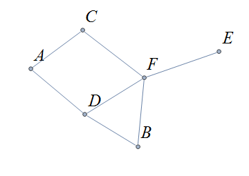
The design of this book is to introduce each concept informally, as was done above for the basic concepts, then notice properties and patterns, generalize what has been noticed, and formalize the ideas to prepare for even deeper analysis.
2.2. Just-In-Time Appendices
Two appendices to this textbook contain additional mathematics that you may need to review as you work your way through the textbook.
In addition, this book contains code snippets written in Python that are designed to aid your understanding of the mathematical concepts. One of the appendices introduces some (but not all) basic concepts from the Python programming language - the goal is to learn "just enough Python" to be able to examine, run, and alter the existing code snippets. You are NOT expected to know the Python programming language before you start this course, and it is NOT one of the goals for you to master Python during this course.
2.3. Applications of Discrete Mathematics
Remixer’s Note: This section is taken from the original “Discrete Math” book, with only a few minor edits.
Discrete mathematics is applied in many areas including the physical, engineering, and increasingly, the social sciences.
2.3.1. Applications to Applied Mathematics
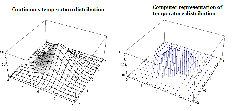
Most problems that involve computational methods, need to be solved using computers. Rather than solve for the temperature map of an entire planar region, we solve for the temperature using a discrete set of mesh or grid of points on a representative subset of the planar region.
2.3.2. Applications to Information Technology and Computer Science
Discrete mathematics is needed for computer science as information and data is stored digitally. Digitally represented data is inherently discrete and is processed using discrete methods. For example a course grid discrete representation of the 2-d temperature distribution from the plate above could be:
\( \left(\begin{matrix}1&1&1\\2&4&8\\3&9&27\\4&16&64\\5&25&125\\\end{matrix}\right) \)
A voter registry may have voters in a database accessible from a list:
\( \left(\begin{matrix}John\ Smith\\Raheem\ Johnson\\.\\.\\.\\Sarah\ Muller\\\end{matrix}\right) \)
Which may need to be accessed and sorted, say geographically or alphabetically.
2.3.3. Applications to Data Science
Data science solutions to many problems use machine learning algorithms that are inherently discrete in nature. The information that needs processing is discrete, as are the basic problems in data science such as classification or clustering problems. In particular
-
Information consisting of data sets is represented using various data structures including graphical structures such as trees. Data science methods and algorithms involve procedures that manipulate these graphical structures to, for example, networks, classification trees, and decision trees.
-
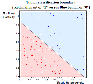
Classification problems are discrete in nature. Classifying tumors as malignant or as benign involves trying to predict if a variable \(Y\) that we can think of as taking on two values either \(0\) or \(1\) either malignant or benign. There are various algorithms used in classification problems, such as the binary tumor classification, including methods from probability.
2.3.4. Applications to Engineering
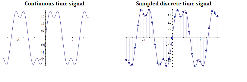
Digital signal processing involves taking a video, audio, or other signal like temperature, pressure, position and velocity, which is continuous, digitizing it and then processing the digital signal mathematically.
2.3.5. Applications of Combinatorics
Combinatorics involves in part the study of counting the number of objects, satisfying a specified condition, from sets of variable size. Enumeration and combinatorics is important in many areas and examples including:
-
Calculating the number of steps an algorithm needs to process a data set of variable size \(𝑛\). This problem is called the computational cost of the algorithm as a function of \(𝑛\).
-
Calculating the possible number of codes in a cryptographic code system
2.3.6. Applications of Graph Theory
Graph theory, which is the study of structures constructed with nodes and the edges joining them, has applications in many fields including,
-
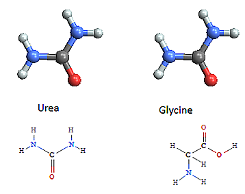
Chemistry - representing molecular bonding and structure
-
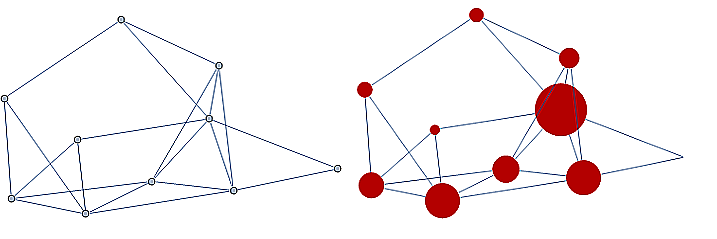
Information technology and computer science - ranking pages on the internet, with pages considered as nodes and page links as edges.
-
Industrial engineering and network optimization
-
Traffic routes (computer, internet, air, highway, subway systems) can be represented with stations as nodes and connections as edges.
-
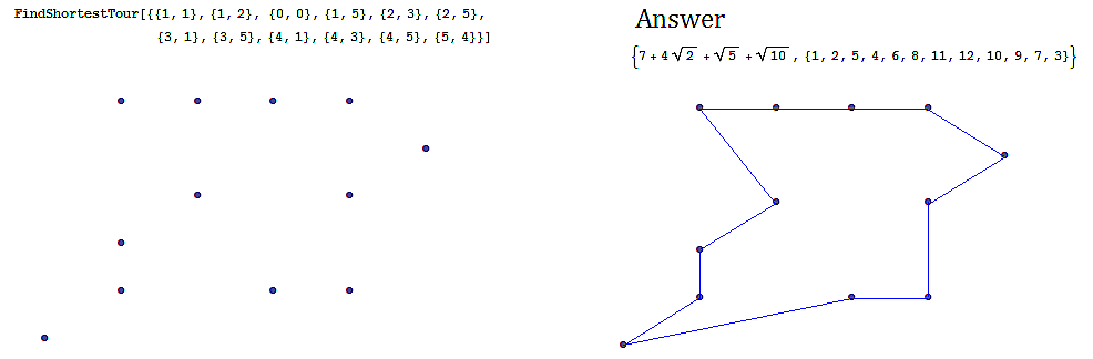
Often we are interested in finding an optimal path in a network such as in the following example, finding the shortest tour over a series of towns on a map.
-
An example of the shortest tour problem, is shown below, using a software solution.
2.3.7. Applications of Probability and Statistics
Many probability assignments are based on counting and combinatorial methods.
-
If we assume that the likelihood of rain is the same on any day in the month of September, we might be interested in the probability that it rains on \(0\) days, it rains on exactly \(1\) day, exactly \(2\) days, etc. Such probability assignments are called discrete distributions, by contrast with continuous distributions like the bell curve.
-
Also probability and statistical techniques are often used in data science. The binary classification problem, of say classifying a tumor as malignant or benign, uses a statistical modeling technique, called regression, specifically logistic regression to determine the strength of the relationship between the independent variable, and dependent heterogeneity variable. In the tumor grading example the independent variable would be \((x_1,x_2 )\) (elastic heterogeneity, nonlinear elasticity), and the dependent variable would be \(Y\), classified as \(0\), or \(1\), (malignant or benign).
2.3.8. Applications to Social Sciences
Discrete mathematical techniques are important in understanding and analyzing social networks including social media networks.
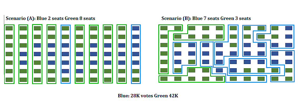
The mathematics of voting is a thriving area of study, including mathematically analyzing the gerrymandering of congressional districts to favor and/or disfavor competing political parties. The following example illustrates some of the fundamental ideas related to gerrymandering.
Consider a fictitious state made up of \(10\) congressional districts with \(7\) thousand voters in each district. To win a district a party (Green or Blue) needs to win \(4\) thousand or more votes. Consider the following two districting map scenarios. In each scenario, the blue party earns \(28\) thousand votes, and the green party earns \(42\) thousand votes. In scenario \(A\), the blue party wins \(2\) out of \(10\) districts, but in scenario \(B\) it wins \(7\) out of \(10\) districts.
3. Set Theory
3.1. Sets
A set is an unordered collection of objects, called elements or members. A set is said to contain its elements. If \(x\) is an element of the set \(S,\) then we write \(x \in S\). If \(x\) is not an element of the set \(S\), then we write \(x \not\in S\).
For example, if \(S\) is the set of states in the United States, then New York is an element of \(S\) and Ontario is not an element of \(S.\) If \(E\) is the set of even integers, then \(2 \in E\) and \(3 \not\in E.\)
There are several different ways to describe a set. One way of describing a set is known as the roster method. This is where we list all the elements of a set between curly braces. For example, \(A = \{1,-2,0,1,-3\}\) is the set whose elements are \(-3\), \(-2\), \(0\), and \(1\). Set \(A\) contains \(4\) members, even though the element \(1\) appears twice in the list. Also, the order of the elements in the list does not matter.
| A WARNING ABOUT THE PYTHON EXAMPLES INVOLVING SETS: The mathematical set \(A = \{1,-2,0,1,-3\}\) is a constant - you cannot change the set by removing elements or inserting new elements. BUT… In Python, objects of type set are mutable so it is possible to remove elements or insert new elements, as shown in the following code example . The correct implementation of mathematical sets in Python uses objects of type frozenset because objects of type frozenset are immutable, just like mathematical sets. But there are advantages to using type set instead: The roster method notation that is used to define a mathematical set can be used to initialize or print a Python set, but cannot be used with a Python frozenset. In particular, we must call the frozenset constructor to create and initialize a frozenset. The authors of the original “Discrete Math” chose to use Python sets instead of frozensets in the code examples; the author of this remix made the same choice. |
Another way of describing a set is the use of set builder notation. We write a set as \[\{x \in D : P(x)\}.\] This is the set of all elements \(x\) from a domain \(D\) that satisfy the predicate \(P(x).\) We can use either the colon \(:\) or the vertical bar \(|\) as the separator in this notation. For example, \(\{ x \in \mathbb{Q} | x^{2} \geq 2 \text{ and } x > 0 \}\) is the set of positive rational numbers that are greater than \(\sqrt{2}\).
Yet another way of describing a set is to use a function or an algebraic expression, as in \[\{ f(x) : x \in D \}.\]This is the set of all values \(f(x)\) for \(x\) in the domain \(D\). For example, \(\{ 2n : n \in \mathbb{N} \}\) is the set of the even natural numbers. Again, we can use either the colon \(:\) or the vertical bar \(|\) as the separator.
We make frequent use of special sets and these are denoted with special symbols.
Other special sets will be defined as needed.
|
When there are too many elements in a set for us to be able to list each one, we often use ellipses (\(\dots\)) when the pattern is obvious. For example, we have \[\mathbb{Z} = \{\dots,-3,-2,-1,0,1,2,3,\dots\}.\] |
3.1.1. Empty Set
Consider the following set described using set builder notation: \[\{x \in \mathbb{Z} : x^2 = 2\}.\]This is the set of all integers whose square is equal to 2. However, no such integers exist. Therefore, using the roster method to describe it, this is the set \(\{ \}.\)
We call the set \(\{ \}\) the empty set and denote this set by \(\emptyset.\) The empty set has no elements.
|
It is important to note that \(\{\}\) and \(\emptyset\) are both ways to write the empty set. However, the mathematical set \(\{ \emptyset \}\) is not the empty set because it contains one element, namely the empty set. In general, the set \(A\) is not the same as the set \(\{ A \}.\) |
|
Python Tip: The mathematical set \(\{ \emptyset \}\) must be implemented as \(\{ \text{frozenset()} \}\), which is the Python set that contains the empty frozenset. In general, anytime we want to implement a mathematical set \(B\) as an element of another mathematical set \(A\) in Python, we need to implement \(B\) as a frozenset in order to be used as an element of the Python set \(A\). This is due to the fact that elements of Python sets must be hashable; further explanation is beyond the scope of this textbook. |
3.1.2. Cardinality
Suppose that a set \(A\) contains a finite number of distinct elements. We refer to the number of elements of \(A\) as the cardinality of \(A\) and denote this by \(|A|\). In this case, we also say that \(A\) is a finite set.
If \(A\) contains an infinite number of distinct elements, we say that \(A\) has infinite cardinality and that \(A\) is an infinite set.
|
The infinity symbol \(\infty\) isn’t used for the cardinality of an infinite set because there are many different infinite cardinal numbers that correspond to the sizes of different infinite sets. It is beyond the scope of this textbook to discuss these infinite cardinal numbers in detail, but as just two examples (1) \(|\mathbb{Q}|\) must be strictly less than \(|\mathbb{R}|\), even though both \(\mathbb{Q}\) and \(\mathbb{R}\) are infinite sets, and (2) perhaps more surprisingly, \(|\mathbb{N}|\) and \(|\mathbb{Q}|\) must be equal even though \(\mathbb{N}\) would appear to be a much smaller set than \(\mathbb{Q}\). |
Thus, we see that \(|\{0,1,2\}| = 3\), \(|\emptyset| = 0\), and \(|\mathbb{Z}|\) is an infinite cardinal number.
3.1.3. Equality
We say that two sets are equal if and only if they contain the same elements. When \(A\) and \(B\) are equal sets, we write \(A = B\). When \(A\) and \(B\) are not equal sets, we write \(A \neq B\).
The sets \(\{2,3,5\}\) and \(\{5,2,3\}\) are equal sets, since they contain the same elements. In fact, \(\{2,3,5\}\) and \(\{5,2,3\}\) are really just two different descriptions of the same set, in the same way that \(2 + 2\) and \(5 - 1\) are two different descriptions of the same number. So we can write \(\{2,3,5\} = \{5,2,3\}\) for the same reason we can write \(2 + 2 = 5 - 1\).
3.1.4. Subsets
We say that a set \(A\) is a subset of a set \(B\) if and only if every element of \(A\) is an element of \(B.\) When \(A\) is a subset of \(B,\) we write \(A \subseteq B\). When \(A\) is not a subset of \(B,\) we write \(A \not\subseteq B\).
In order to show that \(A\) is a subset of \(B,\) we must show that, whenever \(x \in A,\) it is also the case that \(x \in B.\) In order to show that \(A\) is not a subset of \(B,\) we must find a single \(x\) such that \(x \in A\) but \(x \not \in B.\)
Note that, for any set \(A,\) it is always the case that \(\emptyset \subseteq A\) and \(A \subseteq A.\) For any sets \(A\) and \(B,\) if \(A \subseteq B\) and \(B \subseteq A,\) then \(A = B.\)
If \(A \subseteq B\) and \(B\) contains at least one element that is not in A, then we say \(A\) is a proper subset of \(B\), denoted \(A \subset B\).
3.1.5. Power Set
Given a set \(A,\) we refer to the power set of \(A\) as the set of all subsets of \(A.\) The power set of \(A\) is denoted by \(\mathcal{P}(A).\)
|
\(\mathcal{P}(A)\) is a set whose elements are all sets. |
If we let \(A = \{a,b,c\},\) we see that \[\mathcal{P}(A) = \{\emptyset, \{ a \}, \{ b \}, \{ c \}, \{a,b\}, \{a,c\}, \{b,c\}, \{a,b,c\}\}.\] The empty set only has the empty set as a subset. Thus, we see that \[\mathcal{P}(\emptyset) = \{\emptyset\}.\]We can also take the power set of a power set. For example, we have the following:
| \[\begin{split} \mathcal{P}(\{ 1 \}) &= \{\emptyset, \{ 1 \}\},\\ \mathcal{P}(\mathcal{P}(\{ 1 \}) &= \mathcal{P}(\{\emptyset, \{ 1 \})\\ &= \{\emptyset, \{\emptyset\}, \{ \{ 1 \} \}, \{\emptyset, \{ 1 \}\}\}. \end{split}\] |
3.2. Set Operations
We can obtain new sets by performing operations on other sets. When performing set operations, it is often helpful to consider all of our sets as subsets of a universal set \(U.\) We can think of the universal set as the set of all of the objects under consideration.
We can represent set operations visually using Venn diagrams, named after the English mathematician John Venn. A Venn diagram will consist of a rectangle, which represents the universal set, and one or more circles, which represent the sets under consideration. We will then shade in the regions of the diagram that correspond to one or more set operations.
3.2.1. Union
The union of the sets \(A\) and \(B\) is the set containing those elements that are in \(A\) or \(B\) or both, and is denoted by \(A \cup B\). More formally, \[A \cup B = \{x \in U : x \in A \text{ or } x \in B\}.\]
Note that "or" is read here as the "inclusive or". We have the following Venn Diagram for \(A \cup B\):
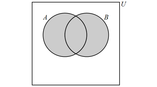
Note that, for any sets \(A\) and \(B,\) \[A \cup B = B \cup A.\]
3.2.2. Intersection
The intersection of the sets \(A\) and \(B\) is the set containing those elements that are in \(A\) and \(B\) and is denoted by \(A \cap B\). More formally, \[A \cap B = \{x \in U : x \in A \text{ and } x \in B\}.\]
We have the following Venn Diagram for \(A \cap B\):
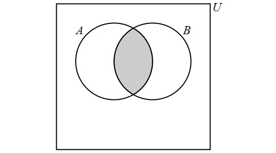
Note that, for any sets \(A\) and \(B,\) \[A \cap B = B \cap A.\] If it is the case that \(A \cap B = \emptyset,\) then we say that \(A\) and \(B\) are disjoint. In other words, two sets are disjoint if and only if they contain no elements in common.
3.2.3. Complement
The complement of a set \(A\) is the set of all elements in the universal set \(U\) which are not elements of \(A\) and is denoted by \(\overline{A}.\) More formally, \[\overline{A} = \{x \in U: x \not\in A\}.\] Note that other textbooks and internet sources may use different notation for the complement of \(A\), such as \(A'\) and \(A^{c}\), but these all stand for the same set, so that \(\overline{A} = A' = A^{c}\).
We have the following Venn Diagram for \(\overline{A}\):
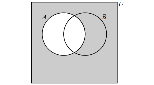
For any set \(A,\) \[ \overline{\overline{A}} = A \] \[ \overline{A} \cup A = U \] + \[ \overline{A} \cap A = \emptyset. \]
3.2.4. Difference
The difference of the sets \(A\) and \(B\) is the set containing those elements that are in \(A\) but not in \(B\) and is denoted by \(A \setminus B\). Set difference is also denoted by \(A - B\). More formally, \[A \setminus B = \{x \in U: x \in A \text{ and } x \not\in B\}.\]
We have the following Venn Diagram for \(A \setminus B\):

Note that, for any sets \(A\) and \(B\), if \(A \neq B,\) then \[A \setminus B \neq B \setminus A.\] However, if \(A = B,\) then \(A\setminus B = B \setminus A = \emptyset\).
3.2.5. Symmetric Difference
The symmetric difference of the sets \(A\) and \(B\) is the set containing those elements that are in \(A\) or \(B\) but not both \(A\) and \(B\). It is denoted by \(A \oplus B\) in this textbook, but other books and sources may use different notation such as \(A \Delta B\). More formally, \[A \oplus B = \{x \in U: (x \in A \text{ and } x \not\in B) \text{ or } (x \in B \text{ and } x \not\in A)\}.\]
We have the following Venn Diagram for \(A \oplus B\):
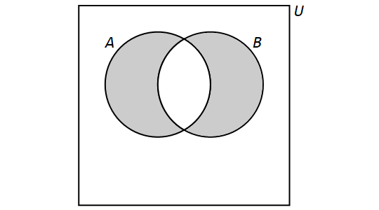
Note that, for any sets \(A\) and \(B,\) \[A \oplus B = B \oplus A.\]
3.2.6. Multiple Set Operations
We can also perform more than one set operation on a collection of sets. For example, let \(A,\) \(B,\) and \(C\) be sets and consider the following set: \[(A \setminus B) \cup (C \setminus B).\]This is the set that is obtained by taking the union of the sets \(A \setminus B\) and \(C \setminus B.\) We have \[(A \setminus B) \cup (B \setminus A) = \{x \in U: (x \in A \text{ and } x \not\in B) \text{ or } (x \in C \text{ and } x \not\in B)\}.\]
We have the following Venn Diagram for \((A \setminus B) \cup (C \setminus B)\):
Note that the Venn Diagram also represents \((A \cup C ) \setminus B\). In general, there are multiple ways to describe the result of multiple set operations.
Video Examples
The following two video examples feature Dr. Katherine Pinzon, Professor of Mathematics at Georgia Gwinnett College.
Video Example 1
Video Example 2
3.2.7. The Cartesian Product
The Cartesian product of two sets \(A\) and \(B\) is the set of ordered pairs defined by,
\( A\times B=\{(a,b)|a\in A \text{ and } b\in B)\}\),
|
Cartesian products are created using ordered pairs, so if \(A\) and \(B\) are different sets, then \(A \times B\) is different from \(B \times A\). |
|
If \(A\) and \(B\) are finite sets, then the cardinality of the Cartesian product \(A × B\) is \(|A × B|=|A| \cdot |B|\). |
|
The Cartesian coordinate systems are natural sets that are naturally Cartesian products. The two-dimensional plane, and the three-dimensional space are represented by the following Cartesian product sets, \(\mathbb{R}^2=\mathbb{R}\times \mathbb{R}=\{(x,y)|x,y\in \mathbb{R}\}\), and, \(\mathbb{R}^3=\mathbb{R}\times \mathbb{R}\times \mathbb{R}=\{(x,y,z)|x,y,z\in \mathbb{R}\}\) |
3.3. Set Identities
Here is a collection of additional properties of the operations on sets. Each of these can be verified by drawing two Venn diagrams, one that represents the left-hand side of the equation and another that represents the right-hand side of the equation and showing that the resulting shadings of the Venn diagrams are the same.
Note that it is traditional to focus on complement, union, and intersection as the three primary set operations because the other operations such as difference and symmetric difference can be written in terms of those three primary operations, for example, \(A \setminus B = A \cap \overline{B}\) and \(A \oplus B = (A \cap \overline{B}) \cup (\overline{A} \cap B)\).
Associative laws: \[ A ∪ (B ∪ C) = (A ∪ B) ∪ C \] \[ A ∩ (B ∩ C) = (A ∩ B) ∩ C \]
Distributive laws: \[ A ∪ (B ∩ C) = (A ∪ B) ∩(A ∪ C) \] \[ A ∩ (B ∪ C) = (A ∩ B) ∪ (A ∩ C) \]
De Morgan’s laws: \[ \overline{A \cup B} = \overline{A} \cap \overline{B} \] \[ \overline{A \cap B} = \overline{A} \cup \overline{B} \]
3.3.1. Operator Precedence (Order Of Operations)
To ensure that we can properly interpret an expression involving multiple set operations, we can either use parentheses or rely on operator precedence.
When an expression for sets involves parentheses, complementation, intersection, and union, we start by evaluating all expressions enclosed in parentheses from left to right, then all complementations from left to right, then all intersections from left to right, and finally all unions from left to right. (Set difference and symmetric difference were left out of this discussion because there does not seem to be a standard definition for where they fit in! But, as shown earlier, those two operations can be rewritten in terms of complementation, union, and intersection.)
For example, the expression \(\overline{A} \cup B \cap C\) represents the same set as \((\overline{A}) \cup (B \cap C)\). Parentheses must be used if you want to represent a different set such as \((\overline{A} \cup B) \cap C\).
This is the same way arithmetic expressions like \(-3 + 5 \cdot 2\) are evaluated: The value of \(-3 + 5 \cdot 2\) is \((-3) + (5 \cdot 2) = 7\), not \((-3 + 5) \cdot 2 = 4\).
3.4. Venn Diagrams, Partitions, and Bitstrings
A partition of a set \(U\) is a set of subsets of \(U\) such that each element \(x \in U\) is a member of exactly one of the subsets in the partition. You already know at least one example of such a partition - the partitoning of the integers \(\mathbb{Z}\) by its 2 subsets in \(\Pi = \{ \text{the set of even integers}, \text{the set of odd integers} \}\); every integer belongs to exactly one of the two elements of the set \(\Pi\).
In fact, for any chosen subset \(A \subseteq U\) we have a partition of \(U\) into the 2 sets that are elements of \(\{ A,\,\overline{A} \}\). Note that each element of \(U\) must be in exactly one of the subsets \(A\) and \(\overline{A}\).
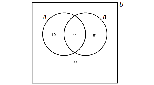
For two subsets \(A\) and \(B\) of a universal set \(U\), consider the Venn diagram of \(A\) and \(B\). By considering all possible intersections of these two sets and their complements, \(U\) is partitioned into 4 subsets, namely, the 4 elements of \(\{ \overline{A} \cap \overline{B},\, \overline{A} \cap B,\,A \cap \overline{B},\,A \cap B \}\). We can refer to each of these 4 subsets by using bitstrings of length 2 as follows:
-
The leftmost bit is 1 if an element of the subset is an element of \(A\), and is 0 if an element of the subset is not an element of \(A\).
-
The rightmost bit is 1 if an element of the subset is an element of \(B\), and is 0 if an element of the subset is not an element of \(B\).
For example, in the following Venn diagram, the subset \(A \setminus B\) is labeled with the bitstring \(10\) because an element of \(A \setminus B\) is an element of \(A\) and not an element of \(B\).
If we had instead three sets \(A\), \(B\), and \(C\), we could partition the universe \(U\) into 8 subsets. In detail, if we have an element \(x \in U\), either \(x \in A\) or \(x \not\in A\), and for each of those possibilities, either \(x \in B\) or \(x \not\in B\), and for each of those possibilities, either \(x \in C\) or \(x \not\in C\). We can apply (twice) the multiplication principle that was first mentioned in chapter 2 to show that there are \(2 \cdot 2 \cdot 2\) possible subsets determined by the Venn diagrams of the 3 sets \(A\), \(B\), and \(C\). Using bitstrings of length 3, we can label these 8 subsets as shown.
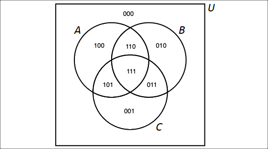
For an integer \(n > 3\), the Venn diagram is less useful for representing the partitioning of the universe created by \(n\) subsets, but we can still reason that there ought to be \(2^{n}\) subsets in the partition, where each of the subsets can be described by a unique bitstring of length \(n\) (We will be able give a formal mathematical proof of this for every positive integer \(n\) later in the textbook after we’ve discussed mathematical induction.)
3.4.1. Disjunctive Normal Form (Set Version)
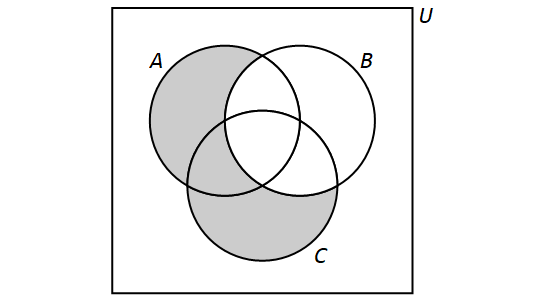
Suppose we have three sets \(A\), \(B\), and \(C\), and have partitioned the universe \(U\) into the 8 subsets as discussed above. Then a set that corresponds to any shading of the Venn diagram can be written as a union of intersections of three sets, with one set chosen from each of the pairs \(\{ A,\,\overline{A} \}\), \(\{ B,\,\overline{B} \}\), and \(\{ C,\,\overline{C} \}\). For example, the set shown in the figure below is equal to \((\overline{A} \cap \overline{B} \cap \overline{C}) \cup (A \cap \overline{B} \cap \overline{C}) \cup (\overline{A} \cap B \cap \overline{C}) \cup (\overline{A} \cap B \cap C)\).
This type of expression is called a disjunctive normal form (or DNF) for the set that it represents. We will see an analog of these in a different context in the chapter on Logic.
3.5. The Principle Of Inclusion-Exclusion (PIE)
In certain application problems, we want to compute the cardinality \(|A \cup B|\) of the union of two given finite sets \(A\) and \(B\). It is tempting to simply add \(|A|\) and \(|B|\), but as the Venn diagram below shows, each element of the intersection \(|A \cap B|\) will be counted twice, once for each bit that is \(1\), if we do so.
The correct relationship between \(|A \cup B|\), \(|A|\), and \(|B|\) is given by \[ |A \cup B| = |A| + |B| - |A \cap B|. \]
Another way to see that this is the correct relationship is to use the partition \(\{ \overline{A} \cap \overline{B},\, \overline{A} \cap B,\,A \cap \overline{B},\,A \cap B \}\) to write
\(| A | = | A \cap \overline{B} | + | A \cap B |\),
\(| B | = | \overline{A} \cap B | + | A \cap B |\), and
\(| A \cup B | = | A \cap \overline{B} | + | A \cap B | + | \overline{A} \cap B |\), so
\(| A | + | B | = | A \cap \overline{B} | + | A \cap B | + | \overline{A} \cap B | + | A \cap B | = | A \cup B | + | A \cap B |\).
If we want to compute the cardinality \(|A \cup B \cup C|\) of the union of three given finite sets \(A\), \(B\), and \(C\), we can again look at the Venn diagram of the partition of \(U\) into 8 sets to see that some of the intersections will be counted one, two, or three times, once for each bit that is \(1\).
We can derive the following formula in much that same way that we did above; in fact, we can just apply the formula we found for two sets to \(| A \cup (B \cup C) |\) and use some of the set identities to help simplify the formula. CSC 230 Spring '24 students at SFSU can see the full derivation in the slide deck Sets part 2 Spring '24. + \[ |A \cup B \cup C| = |A| + |B| + |C| - |A \cap B| - |A \cap C| - |B \cap C| + |A \cap B \cap C|. \]
3.6. Representing Sets as Lists
Remixer’s Note: This section was omitted from the remix since sets can be represented using the types set and frozenset in Python 3.
3.7. Exercises
Remixer’s Note: This section is taken from the original “Discrete Math” book with no changes.
-
Consider as universal set, the set of all \(26\), lowercase letters of the English alphabet, \(U=\{a,b,c,…,v,w,x,y,z\}\), and the sets \(A=\{a,b,c,d,e,f,g,h\}\), \(B=\{f,g,h,i,j,k\}\), and \(C=\{x,y,z\}\). For the sets given below:
-
List the sets below using roster form, and
-
Draw Venn Diagrams for each of the sets
-
\(A\cup B\)
-
\(A\cap B\)
-
\(A\cup C\)
-
\(A\cap C\)
-
\(A \setminus B\)
-
\(B \setminus A\)
-
\(A \setminus C\)
-
\(C \setminus A\)
-
\(A\cup C\)
-
\(A\cap C\)
-
\(\overline{A}\)
-
\(\overline{B}\)
-
\(\overline{C}\)
-
\(\overline{B} \cap \overline{C}\)
-
\( (\overline{A} \cap \overline{B}) \cup (\overline{B} \cap \overline{C})\)
-
-
-
Using Venn Diagrams, determine which of the following are equivalent
-
\(A \setminus (A \setminus B)),\)
\(A\cup B,\) and
\(A\cap B\)
-
\(A\cup \overline{A},\)
\(A\cap \overline{A},\)
\(U,\) and
\(\emptyset\)
-
\(\overline{A}\cap \overline{B}, \)
\(\overline{A\cap B},\)
\(\overline{A}\cup \overline{B},\) and
\(\overline{A\cup B}\)
-
\(A\cup (B\cap C),\)
\(A\cap (B\cup C),\)
\((A\cap B)\cup (A\cap C),\) and
\((A\cup B)\cap (A\cup C),\)
-
\(\overline{\overline{A}\cup(C \setminus B) }),\)
\(A\cap (B \cup \overline{C}),\) and
\(A \setminus (C \setminus B)\)
-
-
Write each of the following sets using set builder notation
-
\(\{\ldots, -9, -7, -5, -3, -2, -1, 1, 3, 5, 7, 9, \ldots \}\)
-
\(\{\ldots, -8, -6, -4, -2, 0, 2, 4, 6, 8, 10,\ \ldots \}\)
-
\(\{ 1, 2, 3, 4, 5, 6, 7, 8, 9, 10 \}\)
-
\(\left\{ 1,\frac{1}{2},\frac{1}{3},\frac{1}{4},\frac{1}{5},\ldots \right\}\)
-
\(\{0, 1, 4, 9, 16, 25, 36, 49, \ldots \}\)
-
\(\{\ldots,-10,-6, -2, 2, 6, 10, 14, 18, 22, \ldots \}\)
-
\(\{ 3, 9, 27, 81, 243,\ldots\}\)
-
\(\{ 1, 9, 25, 49, 81, \ldots \}\)
-
-
Write each of the following sets in roster form
-
\(\{x \in \mathbb{R} : |2x+5|=7\}\)
-
\(\{10n : n \in \mathbb{N}\}\)
-
\(\{10n : n \in \mathbb{Z}\}\)
-
\(\left\{2^n : n \in \mathbb{N}\right\}\)
-
\(\left\{2^n : n \in \mathbb{Z}\right\}\)
-
\(\left\{x \in \mathbb{R} : x^2=4\right\}\)
-
\(\left\{x \in \mathbb{R} : x^3=64\right\}\)
-
\(\left\{x \in \mathbb{Z} : x^2=5\right\}\)
-
\(\left\{x \in \mathbb{R} : x^2= -4\right\}\)
-
\(\left\{x \in \mathbb{Z} : |x-5|=3\right\}\)
-
\(\left\{3n+4 : n \in \mathbb{N}\right\}\)
-
\(\left\{3n+4 : n \in \mathbb{Z}\right\}\)
-
\(\left\{i^n : n \in\mathbb{N}\right\}\), where \(i\) is such that \(i^2=-1\) (the imaginary unit).
-
-
Consider the sets \(A=\{1, 3, 5, 7, 9, 11, 13, 15, 17\}\), \(B=\{2, 5, 7, 11\}\), and \(C=\{1, 2, 3\}\),
-
Determine the cardinalities of following sets,
-
\(|A|\)
-
\(|A\cup B|\)
-
\(|A\cap C|\)
-
\(|\mathcal{P}(A)|\)
-
\(|\mathcal{P}(B)|\)
-
\(|\mathcal{P}(C)|\)
-
-
Give the following power sets,
-
\(\mathcal{P}(B)\)
-
\(\mathcal{P}(C)\)
-
-
-
Determine the cardinalities of following sets,
-
\(\{n \in \mathbb{Z} : |n|\leq 10\}\)
-
\(\{A,B, \emptyset,\{2,5,6\}\}\)
-
\(\{\{A,B\},\{\},\{\{2,5,6\}\},\{\{2,5,6\},C\},\{A,B,C\}\}\)
-
\(\{\{\{A,B\},\emptyset,\{\{2,5,6\},C\},\{A,B,C\}\}\}\)
-
-
Consider the sets, \(B=\{0, 1\}\), \( S=\{spring, summer, fall, winter\}\), and \(C=\{ a, b, c, d,e\}\). For each of the following sets:
-
Determine the following Cartesian products.
-
Calculate the cardinality of each Cartesian product.
-
\(B \times S\)
-
\(S \times B\)
-
\(B \times C\)
-
\(C \times B\)
-
\(B \times B \times B \times B\)
-
\(S \times B \times B\)
-
-
-
Determine the following power sets,
-
\(\mathcal{P}(\{Alabama, Georgia, Florida, Louisiana\} )\)
-
\(\mathcal{P}(\emptyset )\)
-
\(\mathcal{P}(\{\emptyset\} )\)
-
\(\mathcal{P}(\{Alabama \} )\)
-
\(\mathcal{P}(\{Alabama, Georgia, Florida \} )\)
-
\(\mathcal{P}(\{\{Alabama, Georgia \}, \{Florida \} \} )\)
-
-
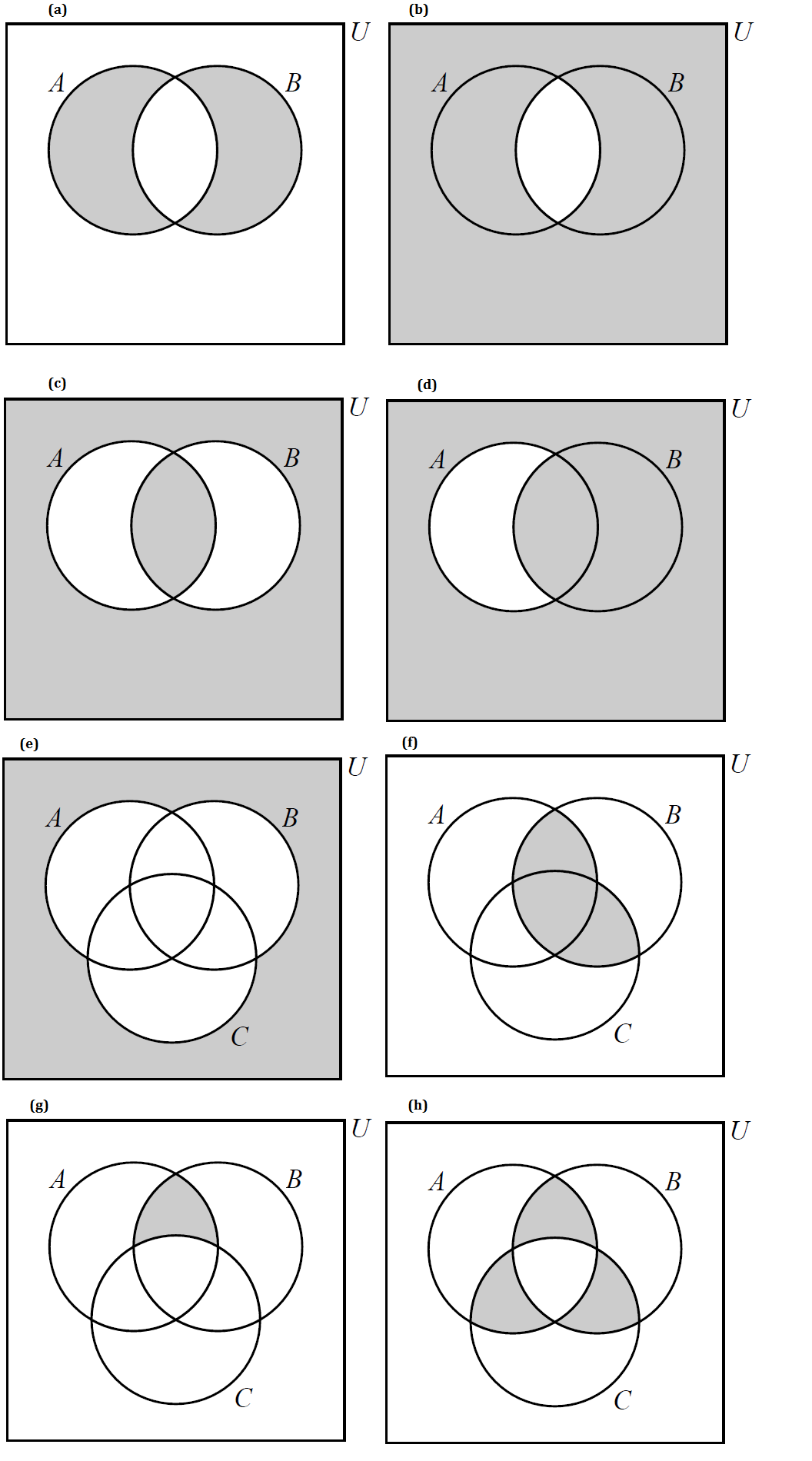
Write the shaded regions in each of the following Venn diagrams using set notation.
-
Determine if each of the following are true or false. Explain your reasoning.
-
\(\{7,4,6,2,11,3,5\}\subseteq \{1,2,3,4,5,6,7,8,9,10,11,12,13\}\)
-
\(\{1,2,3,4,5,6,7,8,9,10,11,12,13\}\subseteq \{7,4,6,2,11,3,5\}\)
-
\(\{7,4,6,2,11,3,5\}\subseteq \{7,4,6,2,11,3,5\}\)
-
\(\{3,8\}\nsubseteq \{7,4,6,2,11,3,5\}\)
-
\( \{3n+4 : n \in \mathbb{N}\} \nsubseteq \mathbb{Z}\)
-
\(\mathbb{N}\subseteq \mathbb{Z}\subseteq \mathbb{Q}\subseteq \mathbb{R}\)
-
\(\{x \in \mathbb{R} : |x|<3\}\subseteq \{x \in \mathbb{R}||x|<5\}\)
-
\(\{x \in \mathbb{R} : |x|>3\}\subseteq \{x \in \mathbb{R}||x|>5\}\)
-
4. Logic
Logic is the study of reasoning. Logic is used to create, analyze, and validate arguments, where an argument is a finite sequence of statements that ends with a conclusion based on inferences made from earlier statements in the argument.
Among the applications of logic to computer science are design of electronic circuits and validation of algorithms and programs.
4.1. Propositional Logic
A proposition is a statement that declares a fact that is either True or False (but not both!)
Propositional logic consists of a set of formal rules for combining propositions in order to derive new propositions.
A goal of propositional logic is to have a method for creating valid arguments that are sequences of propositions, where the correctness and validity of the argument is based solely on the propositions' truth values (True and False), ignoring the actual content of the propositions. Choosing to ignore the actual content of the propositions may seem strange at first, but compare this to doing algebra: We can write \(2 (x + 3 y) = 2x + 6y\) because we know that it is correct and valid to distribute multiplication over addition - we can do the algebra and ignore the actual real-world meaning of the "numerical content" that \(x\) and \(y\) stand for.
In propositional logic, it is traditional to use propositional variables such as p, q, and r to represent the possible assignments of truth values to propositions; often, we refer to the variables themselves as the propositions. Again, compare this to the algebraic example where we can treat \(x\) and \(y\) as numbers even though they are actually variables that stand for numbers.
Logical Translations
A long time ago philosophers discovered we could put our thoughts into symbols and more easily follow lines of reasoning. This was an important step in the eventual development of our modern technological society and our use of digital computers. Before computers can work, we have to put our thoughts into them.
BUT, the English language is difficult and we use many different phrases to represent the same logical statements. Translating statements from English sentences to symbols and back is a skill that needs lots of practice.
We can build compound propositions (also called "propositional functions") from simpler propositions. For example, in the preceding example, we introduced "if p then q" as a new proposition built from the propositional variables p and q.
|
In Python, we use \(\texttt{Boolean}\) variables to represent propositions and define functions for each compound proposition. Each compound proposition can implemented using the \(\texttt{Boolean}\) operations \(\texttt{not}\), \(\texttt{and}\), and \(\texttt{or}\) discussed in the section Operators and Expressions in the chapter "Appendix 0: An Introduction to Python". |
A truth table can be used to show the truth values of compound propositions that are built from other propositional variables. A truth table typically is created with rows representing all possible interpretations of the propositional variables (that is, all possible assignments of truth values to the propositional variables), and columns representing the propositional variables and compound propositions built up from the variables.
4.1.1. Negation
"I am not an astronaut."
The negation of a proposition \(p\), denoted in mathematics by \(\neg p\) and read as "not \(p\)", is the proposition "It is not the case that \(p\)". Note that \(\neg p\) can also be denoted by \(\overline{p}\) or \(\sim \! p.\)
For example, the negation of the proposition "Today is Friday." would be "It is not the case that, today is Friday." or more succinctly "Today is not Friday."
| \(p\) | \(\neg p\) |
|---|---|
True |
False |
False |
True |
From the truth table it can be seen that exactly one of the two propositions \(p\) and \(\neg p\) is True and exactly one is False.
It can also be seen that the two propositions \(p\) and \(\neg (\neg p)\) always have the same truth value.
| In the first few truth tables in this chapter, "True" and "False" are spelled out, but it is more often the case that these words are abbreviated to their first letters, "T" and "F" in truth tables. |
4.1.2. Conjunction
"I am a rock and I am an island."
Let \(p\) and \(q\) be propositions. The conjunction of \(p\) and \(q\), denoted in mathematics by \(p \land q\) and read as "\(p\) and \(q\)", is True when both \(p\) and \(q\) are True and is False otherwise.
| \(p\) | \(q\) | \(p \land q\) |
|---|---|---|
True |
True |
True |
True |
False |
False |
False |
True |
False |
False |
False |
False |
Notice that the two propositions \(p \land q\) and \(q \land p\) always have the same truth value.
4.1.3. Disjunction
"They studied hard or they are extremely bright."
Let \(p\) and \(q\) be propositions. The disjunction of \(p\) and \(q\), denoted in mathematics by \(p \lor q\) and read as "\(p\) or \(q\)", is True when at least one of \(p\) and \(q\) are True and is False otherwise.
| \(p\) | \(q\) | \(p \lor q\) |
|---|---|---|
True |
True |
True |
True |
False |
True |
False |
True |
True |
False |
False |
False |
Notice that the two propositions \(p \lor q\) and \(q \lor p\) always have the same truth value.
4.1.4. Exclusive Disjunction
"Take either 2 Advil or 2 Tylenol."
Let \(p\) and \(q\) be propositions. The exclusive disjunction of \(p\) and \(q\) (also known as xor), denoted in mathematics by \(p \oplus q\), is True when exactly one of \(p\) and \(q\) are True and False otherwise.
| \(p\) | \(q\) | \(p \oplus q\) |
|---|---|---|
True |
True |
False |
True |
False |
True |
False |
True |
True |
False |
False |
False |
Notice that the two propositions \(p \oplus q\) and \(q \oplus p\) always have the same truth value.
|
Exclusive disjunction can be thought of as one or the other, but not both. |
4.1.5. Conditional
"If you get a 100 on the final exam, then you earn an A in the class."
Let \(p\) and \(q\) be propositions. The conditional statement \(p \rightarrow q\), read as "if p then q", "p implies q", or, more formally, "the conditional with hypothesis p and conclusion q", is the proposition that is False when p is True and q is False, and True otherwise. The conditional statement \(p \rightarrow q\) is also called "the implication \(p \rightarrow q\)". Note that \(p \rightarrow q\) can also be denoted by \(p \Rightarrow q\) or \(p \implies q.\) In addition, there are many other ways to express the conditional \(p \rightarrow q\) in English, two of which are "p only if q" and "q if p".
| \(p\) | \(q\) | \(p \rightarrow q\) |
|---|---|---|
True |
True |
True |
True |
False |
False |
False |
True |
True |
False |
False |
True |
|
|
4.1.6. The Converse, Contrapositive and Inverse of a Conditional Statement
Given propositions p and q, we can form three additional compound propositions that are related to the conditional \(p \rightarrow q\):
-
\(q \rightarrow p\), called the converse of \(p \rightarrow q\)
-
\( \neg q \rightarrow \neg p\), called the contrapositive of \(p \rightarrow q\)
-
\( \neg p \rightarrow \neg q\), called the inverse of \(p \rightarrow q\)
The exteneded truth table for the conditional and the three related propositions is shown below.
| \(p\) | \(q\) | \(p \rightarrow q\) (conditional) | \(q \rightarrow p \) (converse) | \( \neg q \rightarrow \neg p\) (contrapositive) | \( \neg p \rightarrow \neg q\) (inverse) |
|---|---|---|---|---|---|
True |
True |
True |
True |
True |
True |
True |
False |
False |
True |
False |
True |
False |
True |
True |
False |
True |
False |
False |
False |
True |
True |
True |
True |
|
From the truth table it can be seen that
|
In the section on logically equivalent propositions we will discuss the bullet points in the preceding note in more detail.
We illustrate these four propositions with an example.
4.1.7. Biconditional
"It is raining outside if and only if it is a cloudy day."
Let \(p\) and \(q\) be propositions. The biconditional \(p \leftrightarrow q\), read as "p if and only if q", is the proposition that is True when p and q have the same truth value, and False otherwise. The biconditional is also called "the bi-implication". Note that \(p \leftrightarrow q\) can also be denoted by \(p \Leftrightarrow q\) or \(p \iff q.\)
| \(p\) | \(q\) | \(p \leftrightarrow q\) |
|---|---|---|
True |
True |
True |
True |
False |
False |
False |
True |
False |
False |
False |
True |
From the truth table it can be seen that the two propositions \(p \leftrightarrow q\) and \(q \leftrightarrow p\) always have the same truth value.
|
The biconditional \(p \leftrightarrow q\) is read as "p if and only if q" because it has the same truth table as the conjunction of the two conditionals "p if q" (that is, \(q \rightarrow p\)) and "p only if q" (that is, \(p \rightarrow q\)). |
It is important to contrast the conditional with the biconditional. Consider the conditional example "If you get a 100 on the final exam, then you earn an A in the class." This means that when you get a 100 on the final you also get an A in the class. The conditional represents a one-way contract: You earn an A in the class if you get a 100 on the final exam. There is nothing said about the result (the grade you earn in the class) if you do NOT meet the condition (get a 100 on the final exam).
As a biconditional the example would say "You get a 100 on the final exam if and only if you earn an A in the class." This becomes a two-way contract: You earn an A in the class if you get a 100 on the final, but you do not earn an A in the class if you do not get a 100 on the final.
4.1.8. Operator Precedence (Order Of Operations)
To ensure that we can properly interpret a compund proposition involving multiple logical operations, we can either use parentheses or rely on operator precedence.
To evaluate a compound proposition, we start by evaluating
-
all expressions enclosed in parentheses from left to right, then
-
all negations from left to right, then
-
all conjunctions from left to right, then
-
all disjunctions from left to right, then
-
all conditionals from left to right, and finally
-
all biconditionals from left to right.
Note that exclusive-disjunction \(\oplus\) was left out of the discussion - this is because different sources assign it different precedences, usually just above or just below the disjunction \(\lor\). For this reason, it’s best to use parentheses whenever \(\oplus\) is present in a compound proposition.
For example, the compound proposition \(\neg p \lor q \land r \rightarrow s\) represents the same proposition as \(((\neg p) \lor (q \land r)) \rightarrow s\). Parentheses must be used if you want to represent a different proposition such as \((\neg p \lor q) \land (r \rightarrow s)\).
4.1.9. Compound Propositions
To find truth values of compound propositions, it is useful to break them up into smaller parts.
When creating your own truth table it is crucial to be systematic about ensuring you have all possible truth values for each of the simple propositions. Each simple proposition has two possible truth values, so the number of rows in the table should be \(2^n\) where \(n\) is the number of propositions. You should also consider breaking complex propositions into smaller pieces.
4.2. Logically Equivalent Propositions
Recall that an interpretation of a proposition is an assignment of truth values to the propositional variables.
Two propositions are considered logically equivalent (or simply equivalent) if they have the same truth values for every possible interpretation. It is often easiest to see this by constructing a truth table for the two propositions and comparing.
We use the symbol \(\equiv\) to denote that two propositions are logically equivalent. So in the preceding example, we would write \(\neg p \lor q \equiv p\rightarrow q\).
| \(\equiv\) is NOT a logical operator used to build compound propositions, but instead is used to say that two propositions are logically equivalent. This is similar to how \(=\) is used in arithmetic: We can write \(2 + 2 = 5 - 1\) to say that \(2 + 2\) and \(5 - 1\) are numerically equivalent, but we don’t use the \(=\) sign as an arithmetic operator to actually do any arithmetic. |
| Saying that two propositions p and q are logically equivalent is the same as saying that the biconditional compound proposition \(p \leftrightarrow q\) is always True. |
4.2.1. Tautologies, Contradictions and Contingencies
A proposition is a tautology if its truth value is always True. That is, a tautology is True for every possible interpretation of its propositional variables.
A proposition is called satisfiable if there is at least one interpretation for which the proposition is True.
A proposition is unsatisfiable if there is no interpretation for which the proposition is True.
A proposition is a contradiction if its truth value is always False. That is, a contradiction is False for every possible interpretation of its propositional variables. This is just another way of saying that it is unsatisfiable.
A proposition that is neither a tautology nor a contradiction is said to be a contingency since its truth value can be either True or False, contingent on the truth value assigned to its propositional variables.
The two compound propositions in the previous example are so important that they have their own names,
4.2.2. De Morgan’s Laws
Two important logical equivalences are De Morgan’s Law. These describe how we "distribute" the \(\neg\) operator across the \(\land\) and \(\lor\) operators.
De Morgan’s Laws can be verified by creating truth tables for \(\neg (p \land q) \leftrightarrow \neg p \lor \neg q\) and \(\neg (p \lor q) \leftrightarrow \neg p \land \neg q\) to show that these propositions are True for every interpretation of \(p\) and \(q\).
4.2.3. Some Other Logical Equivalencies
Here is a collection of additional equivalencies of compound propositions. Each of these can be verified by constructing a truth table to show that the biconditional of the left-hand side and the right-hand side of the logical equivalence is true for all interpretations of the propositional variables.
Double Negation: + \[ p \equiv \neg (\neg p) \]
Commutative laws: \[ p \lor q \equiv q \lor p \] \[ p \land q \equiv q \land p \]
Associative laws: \[ p \lor (q \lor r) \equiv (p \lor q) \lor r \] \[ p \land (q \land r) \equiv (p \land q) \land r \]
Distributive laws: \[ p \lor (q \land r) \equiv (p \lor q) \land (p \lor r) \] \[ p \land (q \lor r) \equiv (p \land q) \lor (p \land r) \]
4.2.4. Disjunctive Normal Form (DNF)
It is traditional to focus on negation \(\neg\), conjunction \(\land\), and disjunction \(\lor\) as the three primary logical operations. This is because any compound proposition can be rewritten in terms of these three operations and the propositional variables present in the original compound proposition.
One way to justify this is by using an expression in disjunctive normal form (DNF), which is a disjunction of one or more conjunctions, where only one of the conjunctions can be true for any interpretation of the propositional variables. This description should become clearer after reading the following example.
4.2.5. Conjunctive Normal Form (CNF)
In some applications of propositional logic, it is more useful to find a logically equivalent expression for a given proposition that is written as a conjunction of several disjunctions. This conjunctive normal form (CNF) can be constructed as shown in the following example.
4.3. Predicates and Quantifiers
4.3.1. Predicates
A predicate is a statement that includes one or more variables such that when values are assigned to the variables the predicate becomes a proposition.
Predicates are denoted as \(P(x)\) or \(Q(x,y)\) where \(P\) and \(Q\) represent the statements and \(x\) and \(y\) are variables. After a value is assigned to each variable, the predicate becomes a proposition which has a truth value. That is, we "evaluate" a predicate by substituting inputs into the variables and get a proposition as the output.
4.3.2. Quantifiers
Consider the statements
-
For all integers \(x\), \(x^2\geq 0\).
-
Some student in the class has a birthday in July.
Each of these statements considers a proposition over an entire population or set, called the domain, and quantifies how many elements (or people) in the set satisfy the proposition. To represent this idea, we use two main quantifiers, the universal quantifier and the existential quantifier.
The Universal Quantifier, \(\forall\), represents the statement "for all", "for every", "for each". When it comes before a statement, it means that statement is true for all values in the domain.
The Existential Quantifier, \(\exists\), represents the statement "there exists", "for some", "at least one". When it comes before a statement, it means the statement is true for at least one value in the domain.
Recall the previous example statements:
-
For all integers \(x\), \(x^2 \geq 0\).
Let \(P(x)\) be the predicate "\(x^2 \geq 0\)". Then we write the statement as \(\forall x P(x)\), where the domain is the set of all integers. This quantified statement will be true since anytime you square a nonzero integer it is positive and \(0^2=0\).
-
Some student in the class has a birthday in July.
Let \(Q(s)\) be the predicate "student \(s\) has a birthday in July". Then we write the statement as \(\exists s Q(s)\), where the domain is the set of all students in the class. This statement will be true as long as at least one student in the class has a birthday in July. It will be false, otherwise.
4.3.3. Negation of Quantifiers
It is important to consider the negation of a quantified expression.
-
"Every student in this class has taken Programming Fundamentals."
This is a universally quantified statement and can be expressed as \(\forall x P(x)\) where \(P(x)\) is the statement "\(x\) has taken Programming Fundamentals" and the domain consists of all the students in this class. The negation of the statement would be "It is not true that every student in this has taken Programming Fundamentals." Equivalently,
-
"There is a student in this class who has NOT taken Programming Fundamentals."
This is an existentially quantified statement expressed as \(\exists x \neg P(x)\).
This demonstrates that the negation of a universally quantified statement is an existential statement. In symbols, we have \(\neg \forall x P(x)\equiv \exists x \neg P(x)\).
Similarly, the negation of an existential statement is a universal statement. \(\neg \exists x P(x) \equiv \forall x \neg P(x)\).
The predicate of a quantified statement could be a compound statement. For instance,
-
Some dogs are big and fluffy.
This is written as \(\exists x (B(x) \land F(x))\) where \(B(x)\) is the proposition "\(x\) is big." and \(F(x)\) is the proposition "\(x\) is fluffy." and the domain is dogs. Negating this statement would give
\(\neg \exists x (B(x) \land F(x)) \equiv \forall x \neg (B(x) \land F(x)) \equiv \forall x (\neg B(x) \lor \neg F(x))\)
In words,
-
All dogs are not big or not fluffy.
4.3.4. Nested Quantifiers
There are times it will take more than one quantifier to express a statement.
-
For all integers \(x\), there exists an integer \(y\), such that \(x+y=0\).
This statement contains both a universal and an existential quantifier. \(\forall x \exists y S(x,y)\) where \(x\) and \(y\) are integers and \(S(x,y)\) is the proposition \(x+y=0\). This statement means, if you have any integer \(x\) (for instance \(x=5\)) then you can find an integer \(y\) (for instance \(y=-5\)) such that \(x+y=0\).
The order of the quantifiers matters. \(\exists x \forall y S(x,y)\) would be
-
There exists an integer \(x\), such that for all integers \(y\), \(x+y=0\).
Note that in this statement you find an integer \(x\) so that when you add any integer \(y\) to it you always get 0.
The first statement, for all integers \(x\), there exists an integer \(y\) such that \(x+y=0\), is true. For any integer \(x\) you could choose \(y=-x\) and \(x+y=x+(-x)=0\). While the second statement, there exists an integer \(x\), such that for all integers \(y\), \(x+y=0\), is false.
To negate nested quantifiers, repeatedly apply De Morgan’s Laws of negating a quantifier and a predicate.
Namely, \(\neg \forall x P(x) \equiv \exists x \neg P(x)\) and \(\neg \exists x P(x) \equiv \forall x \neg P(x)\).
4.4. Applications of Logic
Remixer’s Note: This section is taken from the original “Discrete Math” book with no changes.
In this section we consider two applications of logic to information technology and computer science. The first involves bitwise operations, and the second designing and analyzing logic circuits.
4.4.1. Bitwise operations
A bitwise operation is a Boolean operation that operates on the individual bits (\(0s\), or \(1s\)) of the operand(s) and are summarized
We summarize the truth tables for the bitwise boolean operators.
| \(p\) | \(q\) | \(AND\) & | \( \ OR\ | \) | \(XOR\) \({}^{\wedge}\) | \(IF\) \(\Rightarrow\) | \(IFF\) \(\Leftrightarrow\) |
|---|---|---|---|---|---|---|
1 |
1 |
1 |
1 |
0 |
1 |
1 |
1 |
0 |
0 |
1 |
1 |
0 |
0 |
0 |
1 |
0 |
1 |
1 |
1 |
0 |
0 |
0 |
0 |
0 |
0 |
1 |
1 |
4.4.2. Logic Circuits
Logic circuits are important in designing the arithmetic and logic units of a computer processor. Consider the problem of adding two \(8\)-bit numbers in binary. In binary \(0+0=0\), and \(1+0=0+1=1\), but, as in decimal addition, in binary \(1+1=2\), which in binary will be a sum of \(0\) and a carry of \(1\) to the next significant column on the left. Thinking then of adding a specific column of two binary digits, say \(A\) and \(B\), involves as input the digits \(A, B\) and the carry in from the previous column say \(C_{in}\). The output will be the sum \(S\) and the carry out to the next column, say \(C_{out}\). These are the basic components of what is called a binary adder.
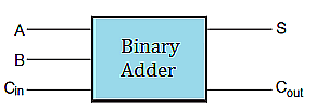
The logic table for binary addition based on the digital inputs \(A, B, C_{in}\), and digital outputs \(S\) and \(C_{out}\) is summarized in the table.
| \(A\) | \(B\) | \(C_{in}\) | \(\mathbf{S}\) | \(\mathbf{C_{out}}\) |
|---|---|---|---|---|
1 |
1 |
1 |
\(\mathbf{1}\) |
\(\mathbf{1}\) |
1 |
1 |
0 |
\(\mathbf{0}\) |
\(\mathbf{1}\) |
1 |
0 |
1 |
\(\mathbf{0}\) |
\(\mathbf{1}\) |
1 |
0 |
0 |
\(\mathbf{1}\) |
\(\mathbf{0}\) |
0 |
1 |
1 |
\(\mathbf{0}\) |
\(\mathbf{1}\) |
0 |
1 |
0 |
\(\mathbf{1}\) |
\(\mathbf{0}\) |
0 |
0 |
1 |
\(\mathbf{1}\) |
\(\mathbf{0}\) |
0 |
0 |
0 |
\(\mathbf{0}\) |
\(\mathbf{0}\) |
It can be shown that the logic for the outputs \(S\), and \(C_{out}\) is given by the following propositions \[ C_{out}=(A\land B)\lor \left(B\land C_{in}\right)\lor \left(A\land C_{in}\right)\] \[S=\left(\sim A\land \sim B\land C_{in}\right)\lor \left(\sim A\land B\land \sim C_{in}\right)\lor \left(A\land \sim B\land \sim C_{in}\right)\lor \left(A\land B\land C_{in}\right) \]
Implementing these logical outputs based on the inputs \((A,B, C_{in})\), is through the use of electronic circuits called logic gates.
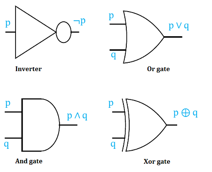
The basic logic gates, are the Inverter or Not gate, the And gate, the Or gate and the Xor gate. The graphical representation for each is shown below.
We end this section by first analyzing logic circuits to give their outputs in terms of their input variables, and then, constructing logic circuits based on logical statements.
Determine the output of the following logic circuit in terms of the input variables, \(p, q\), and \(r\).
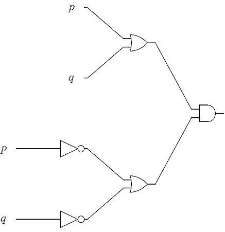
Proceeding left to right, determine the output of the leftmost gates first using the basic gate outputs.
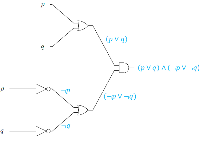
The output of the logic circuit is \( ( p \lor q)\land ( \neg p \lor \neg q)\)
In the next two examples, we design logic circuits based on logical propositions. The idea is to work backward using order of operations from the right to the left.
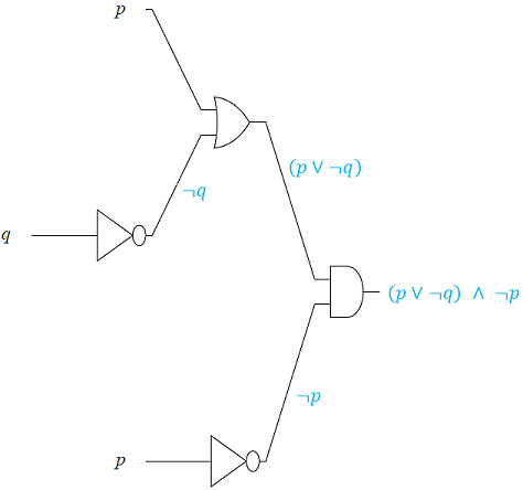
Design a logic circuit for \((p\vee\lnot\ q)\land\lnot\ p\).
Working backwards from right to left we have the following sequence of gates
1) An AND gate \((p\vee\lnot\ q)\underline{\land} \lnot\ p\).
2) The inputs to the AND gate are \((p\vee\lnot\ q)\) and \(\lnot\ p\).
3) These inputs come from the output of an INVERTER, for \(\underline{\lnot}\ p\) and an OR gate \((p \underline{\vee}\lnot\ q)\).
4) There are two inputs to the OR gate \((p \underline{\vee}\lnot\ q)\), being \(p\), and the output of an INVERTER, \(\underline{\lnot} q\).
Putting these now in left to right order we obtain the following logic circuit.
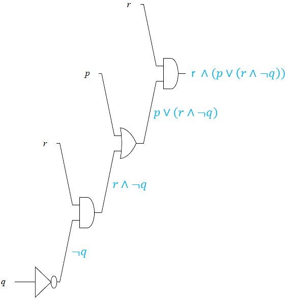
Design a logic circuit for \(r\land (p\lor (r\land \neg q))\).
Working backwards from right to left we have the following sequence of gates
1) An AND gate \(r\underline{\land} (p\lor (r\land \neg q))\).
2) The inputs to the AND gate are \(r\) and \(p\lor (r\land \neg q)\).
3) The input, \(p\lor (r\land \neg q)\), comes from the output of an OR gate for \(p \underline{\lor} (r\land \neg q)\).
4) The inputs to the OR gate, \(p \underline{\lor} (r\land \neg q)\), are \(p\) and \((r\land \neg q)\), which is an AND gate.
5) The inputs to the AND, gate, \(r \underline{\land} \neg q\), are \(r\) and the output of an INVERTER, \(\underline{\neg} q\).
Putting these now in left to right order we obtain the following logic circuit.
4.5. Exercises
Remixer’s Note: This section is taken from the original “Discrete Math” book with no changes.
-
Which of these statements are propositions? Explain your reasoning
-
Is Atlanta the capital of Georgia?
-
All birds fly
-
\(2\ \times\ \ 3\ =\ 5\)
-
\(5\ +\ 7\ =\ 7+5\)
-
\(x\ +\ 2\ =\ 11\)
-
Answer this question.
-
The rain in Spain
-
-
Construct truth tables for,
-
\(a\vee b\Rightarrow\lnot b\)
-
\((a\vee\lnot b)\ \Leftrightarrow\ a\)
-
\((a\Rightarrow b)\ \bigwedge\ (b\ \bigwedge\ \lnot c)\)
-
\((a\ \bigvee\ b)\ \Rightarrow\ (\ \lnot c\ \bigvee\ a)\)
-
\((a\ \bigvee\ b)\ \bigwedge\ (c\ \bigvee\lnot d\ )\)
-
\((\lnot c\ \bigwedge\ \ b)\ \bigvee\ \ (a\Rightarrow\ \lnot d\ )\)
-
-
Using truth tables, determine if each of the following is a tautology, contradiction, or neither (conditional)
-
\(\neg ((a\lor b)\lor (\neg a\land \neg b))\)
-
\(\left(\left(a\vee b\right)\land\lnot a\right)\Rightarrow b\)
-
\(\left(\left(a\vee b\right)\land a\right)\Rightarrow b\)
-
\(p\land r)\lor (\neg p\land \neg r)\)
-
\(\neg ((p\lor q)\lor (\neg p\land (\neg q\lor r)))\)
-
\(\neg (p\land q)\lor (q\lor r)\)
-
-
Using truth tables determine which of the following are equivalent
-
\(\left(p\Rightarrow q\right)\Rightarrow r\),
\(\left(p\land\lnot q\right)\vee r,\) and
\(\left(p\land\lnot q\right)\land r\)
-
\((a\lor b)\land c,\)
\((c\land a)\lor (c\land b),\) and
\(\neg ((\neg a\land \neg b)\lor \neg c)\)
-
-
Let \(C(x)\) be the statement "\(x\) has visited Canada." where the domain consists of the students at GGC. Express each of the quantifications in English.
-
\(\exists x C(x)\)
-
\(\forall x C(x)\)
-
How would you determine whether each of these statements is true or false?
-
-
Determine the truth value of each of these statements if the domain for all variables, \(m , n\) is the set of all integers, \(\mathbb{Z}\), explaining your reasoning.
-
\(\forall n:\left(n^2\geq 1\right)\)
-
\(\forall n:\left(n^2\geq 0\right)\)
-
\(\ \exists\ n:(n^2=3)\)
-
\(\ \exists\ m\forall\ n:(m+n=n-m)\)
-
\(\forall\ n\exists\ m:\ (n\cdot\ m=m)\)
-
\(\ \exists\ n\forall\ m:\ (n\cdot\ m=m)\)
-
\(\ \exists\ n\forall\ m:\ (n\cdot\ m=n)\)
-
-
Consider each of the compound propositions. (i) Translate each using logical symbols and letters, stating what each letter represents, (ii) Negate each using plain English sentences, and (iii) Translate the negated statements using logical symbols and quantifiers.
-
If it snows today, then I will go skiing tomorrow.
-
Mei walks or takes the bus to class.
-
Every person in this class understands mathematical induction.
-
In every mathematics class there is some student who falls asleep during lectures.
-
There is a building on the campus of some college in the United states in which every room is painted white.
-
-
Let \(p\), be the proposition ”My bicycle needs a tire replaced,” \(q\), be the proposition ”I will go cycling”, and, \(r\), be the proposition ”Rain is in the forecast.”
-
Express each of these compound propositions using plain English sentences.
-
\(\neg p\vee q\)
-
\(\neg p\Rightarrow \neg q\)
-
\((\neg p\wedge r)\Rightarrow q\)
-
\((\neg p\wedge r)\Rightarrow q\)
-
\((\neg p\wedge q)\vee r\)
-
-
Write these compound propositions using \(p\), \(q\) and, \(r\) and logical connectives (including negation).
-
If my bicycle tire does not replacement I will go cycling.
-
My bicycle tire does not replacement, there is rain in the forecast but I will go cycling
-
Whenever there is rain in the forecast, I do not go cycling.
-
If there is rain in the forecast or my tire needs replacement I will not go cycling.
-
Rain is not forecast whenever I go cycling.
-
Rain is not forecast and my tire does not need replacement whenever I go cycling.
-
-
-
Design logic circuits with the following output
-
\((p\lor (q\land \neg r))\lor \neg (p\land q)\)
-
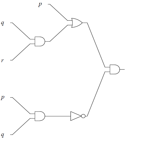
\((p\lor (q\land r))\land \neg (p\land q)\)
-
-
Consider the predicate \(Q(x,y): x\ \cdot\ y=5\), where the domain of \(x\) and \(y\) is all positive real numbers \(\mathbb{R}^+\), or \(x,\ y\ >0\). Determine the true value of the following, an explain your reasoning.
-
\(Q(1,5)\)
-
\(Q\left(2,\frac{5}{2}\right)\)
-
\(\exists\ y,\ Q\left(7,y\right)\)
-
\(\ \forall\ y,\ Q\left(7,y\right)\)
-
\(\exists\ x\ \forall\ y,\ Q\left(x,y\right)\)
-
\(\ \forall\ \ x\ \exists\ \ y,\ Q\left(x,y\right)\)
-
-
Consider the predicate \(R(x,y):\ 2x+y=0\), where the domain of \(x\) and \(y\) is all rational numbers, \(\mathbb{Q}\). Determine the true value of the following, an explain your reasoning.
-
\(R(0,0)\)
-
\(R(2,-1)\)
-
\(R\left(\frac{1}{5},-\frac{2}{5}\right)\)
-
\(\exists y,\ R\left(0.2,y\right)\)
-
\(\ \forall y,\ R\left(7,y\right)\)
-
\(\exists\ x\forall\ y,\ R\left(x,y\right)\)
-
\(\ \forall\ x\ \exists\ y,\ R\left(x,y\right)\)
-
-
Calculate the bitwise \(AND\), the bitwise \(OR\), and the bitwise \(XOR\) of the following pairs of bytes, or sequence of bytes
-
\(01111111\) and \(11101001\)
-
\(1110010111111010\) and \(0101110101100011\)
-
-
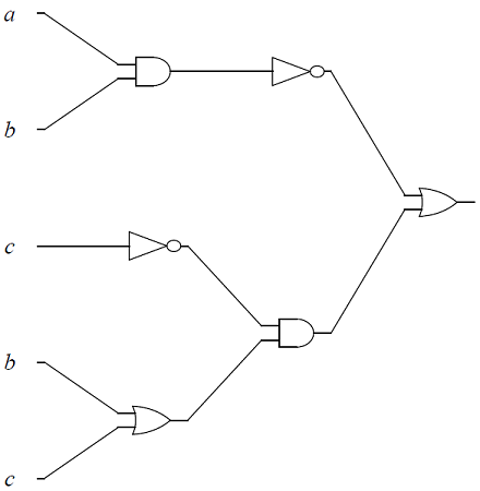
Give the output for each of the logic circuits in terms of the input variables,
-
The logic circuit, with input variables, \(p, q\), \(r\).
-
The logic circuit, with input variables, \(a, b\), \(c\).
-
-
Design a logic circuit for \(r\land (p\lor (r\land \neg q))\).
5. Proofs
Recall from the chapter on Logic that an argument is a finite sequence of statements that ends with a final statement, the conclusion, that is based on inferences made from the earlier statements, called premises.
An argument is valid if it is of a form such that if all premises are True then the conclusion must be True, too. An argument is not valid just because it exists! Compare this situation to a proposition, which is a single statement that may be either True or False (but not both); an argument is a finite sequence of statements that may be either valid or invalid.
A proof is a valid argument made up of propositions. In a proof, some premises may be axioms or postulates, which are propositions that we simply ASSUME to be True. Other premises used in a proof may be previously-proven propositions called theorems. There are many other terms used for theorems depending on the context, such as lemma (a minor theorem needed to prove a more important major theorem) and corollary (a theorem that is a conclusion based on a premise that is a more important theorem), but each of these specialized terms describes a theorem.
5.1. Rules Of Inference
To create a proof, we must proceed from True propositions to other True propositions without introducing False propositions into the argument. To do this, we use rules of inference, which are ways to draw a True conclusion from one or more premises that are already known to be True (or assumed to be True). That is, a rule of inference is an argument form that corresponds to a tautology, and so is valid.
In the following subsections we will discuss some of the more common rules of inference.
5.1.1. Transitivity Of The Conditional
The following rule of inference is called pure hypothetical syllogism, but we will use the less formal name transitivity. It is the basis of conditional proof in mathematics.
By applying transitivity multiple times, we can build a finite chain of implications of any length we want:
-
\(p \rightarrow p_{1}\)
-
\(p_{1} \rightarrow p_{2}\)
-
\(p_{2} \rightarrow p_{3}\)
-
\(\vdots\)
-
\(p_{k-1} \rightarrow p_{k}\)
-
\(p_{k} \rightarrow r\)
-
\(\therefore p \rightarrow r\)
5.1.2. Rules Of Inference And Fallacies Arising From The Conditional
Recall that if we have propositions p and q, we can form the conditional with hypothesis \(p\) and consequent \(q\), written as \(p \rightarrow q\), as well as three other related conditionals.
-
\(p \rightarrow q\), the conditional
-
\(q \rightarrow p\), the converse of \(p \rightarrow q\)
-
\(\neg q \rightarrow \neg p\), the contrapositive of \(p \rightarrow q\)
-
\(\neg p \rightarrow \neg q\), the inverse of \(p \rightarrow q\)
Also, recall that \((p \rightarrow q) \equiv (\neg q \rightarrow \neg p)\). That is, \((p \rightarrow q) \leftrightarrow (\neg q \rightarrow \neg p)\) is a tautology. This means that the conditional is logically equivalent to its contrapositive. The conditional is NOT logically equivalent to either its converse or its inverse, as was shown using truth tables in the Logic chapter.
From the four conditionals we get two rules of inference and two fallacies. Together, these four argument forms are referred to as the mixed hypothetical syllogisms.
First, here are the two rules of inference.
Next, here are the two fallacies. They are included because they are very common errors to be aware of and to avoid.
The following image uses an Euler diagram of two sets \(A \subseteq B\) to explain why the converse error is a fallacy. The image can also be used to explain why the inverse error is a fallacy.
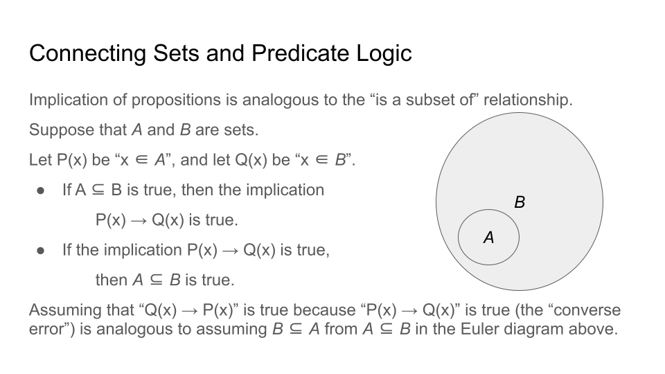
Suppose you were told that \(c\) is an element of \(B\) in the preceding image. Can you determine whether \(c\) is an element of \(A\), too?
5.1.3. Other Common Rules Of Inference
Any tautology of the form \(p \rightarrow q\) can be used to define a rule of inference. In particular, we can define a rule of inference corresponding to the tautology \((p_{1} \land p_{2} \land \ldots \land p_{n})\rightarrow p_{1}\) for each integer \(n \geq 1\). This means that there are at least as many possible tautologies as there are natural numbers! How do we deal with infinitely many tautologies?
In general, there is a small number of rules of inference that are used in most proofs. Proofs often are built up to a large size by applying just a few rules of inference multiple times.
Here are some of the more commonly-used rules of inference. In the remix author’s opinion, it’s better to practice using these rules of inference rather than to focus on memorizing them as formal rules with special names.
There are many more rules of inference we could write down and give names to. Instead, we’ll just list a few tautologies.
5.2. Proof Techniques - SECTION IN PROGRESS
In this section we will give several examples of formal mathematical proofs to illustrate different techniques.
Each proof starts with us stating a conjecture, which is a proposition with undetermined truth value. The goal of each proof is to determine the truth value of the relevant conjecture.
To simplify the description of the proof techniques, we’ll only consider the case where the proof has a single premise \(p\), that is, we’ll always assume that our proof involves a single conditional \(p \rightarrow q\). This may seem like an oversimplification, but it is not: We are simply renaming the conjunction \((p_{1} \land p_{2} \land \ldots \land p_{n})\) of the actual premises by using the single propositional variable \(p\), that is we are defining \(p\) by the logical equivalence \(p \equiv (p_{1} \land p_{2} \land \ldots \land p_{n})\)
MORE TO COME!!
6. Mathematical Induction
Mathematical induction is a proof technique that is used to prove infinitely many propositions using only two steps, where each of the steps is of finite length (in terms of time, symbols, words, phonemes, etc.). Recall that a proof consists of finitely many propositions, where each proposition has a finite length.
6.1. Why Is Mathematical Induction Needed?
In the preceding example, we could imagine running the code for each positive integer value of \(n\), but this would require an infinite number of runs and/or using a loop that must execute an infinite number of times. If we could find a pattern linking the computed result for one integer to the result computed for the next largest integer, we could try to use that to justify that the code will always work without needing to run it for every value of \(n\). The following example illustrates how we can do this.

The preceding image shows \(16\) colored "balls" arranged as a square.
Consider the predicate \(P(n)\): "The sum of the first \(n\) positive odd integers is equal to \(n^{2}\)." Recall that a predicate is a function that maps each input in the predicate’s domain to a proposition.
In the following code snippet, function \(P\) implements the predicate used in this example. Recall that the predicate’s output is the proposition itself, but the output does not indicate whether that proposition is true of false.
Think about how the image can be used to prove that each of the following four propositions is true.
-
\(P(1)\): "The sum of the first \(1\) positive odd integers is equal to \(1^{2}\)." (I know, this is not proper US English!)
-
\(P(2)\): "The sum of the first \(2\) positive odd integers is equal to \(2^{2}\)."
-
\(P(3)\): "The sum of the first \(3\) positive odd integers is equal to \(3^{2}\)."
-
\(P(4)\): "The sum of the first \(4\) positive odd integers is equal to \(4^{2}\)."
How can you change the image so that it could be used to prove that \(P(5)\) is true, too ? How would you need to change the image to prove that \(P(n)\) is true for every possible choice for the positive integer \(n\) ? Note that stating a conjecture such as "It seems like it must be true for any positive integer \(n\)" is not a valid mathematical proof !
To prove that \(P(n)\) is true for every positive integer \(n\) using images, we need either an infinite number of images (one image for each positive integer \(n\)) or one image of an infinitely large "square". Notice that neither of these options gives a proof of finite length.
The following code could be used to prove \(P(n)\) for many more values of \(n\), but we would eventually run into constraints based on time and computing resources.
Use the Next button to step through the program below.
To prove that \(P(n)\) is true for every positive integer \(n\) using the code, we need one output from the function for each positive integer \(n\), that is, we would need an infinitely long proof, which is infeasible.
For example, if you needed to convince someone that the proposition \(P(1,\!000,\!000)\) must be true by drawing the complete image for that value of \(n\), you would draw a square with \(1,\!000,\!000\) rows each containing \(1,\!000,\!000\) balls, for a total of \(1,\!000,\!000,\!000,\!000\) balls. And then what if that person asked you to prove that \(P(1,\!000,\!000,\!000,\!000\))$ is true ?!?!? Even the code would likely fail to prove this unless you have a lot of time and computing resources available.
This is why mathematical induction is used: The induction step justifies that we can (in principle) complete as large a finite number of these proofs as we need to by assuming we already have drawn the \(k \times k\) square of balls to prove that \(P(k)\) is true then we can use the pattern suggested in the image to enlarge the square to a \((k+1) \times (k+1)\) square of balls that proves \(P(k+1)\) must be true. Or, in terms of the Python code, we already can prove that the output for input int \(k\) is a square, and can show that this implies that the output for input int \(k+1\) is also a square.
That is, we could write down as large a finite number of proofs as we need to prove \(P(n)\) for a specifically chosen value of \(n\)… but since there is no bound on this chosen value of \(n\), we in fact have proven the predicate \(P(n)\) for all positive values of \(n\).
| Mathematical induction does NOT state that we can write a single proof of \(\forall n P(n)\) but instead let’s us justify that we can in principle write down a proof of \(P(n)\) for every possible value of \(n\). To clarify, if we first choose a specific value for the integer \(n\), then we can write a proof of \(P(0)\) (and stop if \(n = 0\)), and then write a proof of \(P(1)\) that builds on the proof of \(P(0)\) (and stop if \(n = 1\)), and then write a proof of \(P(2)\) that builds on the proof of \(P(1)\) (and stop if \(n = 2\)), and so on, until we have written a proof of \(P(n)\) that builds on the proof of \(P(n-1)\). |
We will prove that the predicate \(P(n)\) is true for all positive integers \(n\) - in this case it does not make sense to have ``the sum of the first \(0\) positive integers'', so the basis step will use \(n=1\), which corresponds to the single red ball in the image, instead of \(n=0\), which would correspond to \(0\) balls.
Basis Step: In this case, the basis corresponds to \(n=1\). \(P(1)\) is the proposition ``The sum of the first \(1\) positive odd integers is equal to \(1^{2}\).''
\(P(1)\) is a true proposition since \(1 = 1^{2}\) (Note that the only term in the sum on the left-hand side of the equation is \(1\)). The predicate \(P(n)\) is true for \(n=1\).
It may seem a bit strange to use "the sum of the first \(1\) odd integers", so we can do an additional basis step for \(n=2\). THIS IS NOT NECESSARY, but may aid in seeing the pattern. \(P(2)\) is the proposition ``The sum of the first \(2\) positive odd integers is equal to \(2^{2}\).''
Induction Step: We will assume that the proposition \(P(k)\) is true and prove that \(P(k+1)\) must also be true. In this context, the proposition \(P(k)\) is called the induction hypothesis (and \(P(k+1)\) could probably be called the induction conclusion, but I’ve never seen anyone use that name).
Now, how do we generalize the pattern seen in the image of the \(16\) "balls" ? Well, suppose we have a \(k \times k\) square arrangement of such balls… how do we add in the new gnomon of balls to increaese the square to \((k+1) \times (k+{1)}\) ? We can add a new row of \(k\) balls at the top, and a new column of \(k\) balls to the right, and then \(1\) additional ball at the upper right. So, as an algebraic equation, we’d like to show that \(k^{2} + k + k + 1 = (k+1)^{2}\).
That is, assume that \(P(k)\) is true, where \(k\) is some unspecified positive integer (again, this is called the inductive hypothesis). Based on the formula for the \(k\text{th}\) odd positive integer, we can rewrite \(P(k)\) as the equation \[1+3+…+(2k-1) = \sum\limits_{i=1}^{k}(2i-1) = k^{2}.\]
Now we prove that this implies \(P(k+1)\) is true. That is show + \[\sum\limits_{i=1}^{k+1}(2i-1) = \left(\sum\limits_{i=1}^{k}(2i-1)\right) + (2(k+1)-1) = k^{2} + (2(k+1)-1)\] where we have substituted \(k^{2}\) for the sum \(\sum\limits_{i=1}^{k}(2i-1)\) based on the inductive hypothesis.
Now we simplify this using algebra and show that it is the same as the right hand side. + \[\sum\limits_{i=1}^{k+1}(2i-1) = k^{2} + (2(k+1)-1) = k^{2} + 2k + 2 - 1 = k^{2} + 2k + 1 = (k+1)^2.\]
We have proven that the equation \(1+3+...+(2k-1) = \sum\limits_{i=1}^{k}(2i-1) = k^{2}\) implies the equation \(1+3+...+(2k-1) + (2k+1) = \sum\limits_{i=1}^{k+1}(2i-1) = (k+1)^{2}\), that is, \(P(k) \rightarrow P(k+1)\).
Conclusion of the proof: We have proven both the basis step and the induction step, therefore, \(1+3+...+(2n-1) = \sum\limits_{i=1}^{n}(2i-1) = n^{2}\) for all positive integers \(n\).
We can now formalize what we did in the example above. Suppose that we have a predicate \(P(n)\) that is defined for all \(n \in \mathbb{N}\), that is, \(P\) is a function that maps each natural number to a corresponding proposition, and that we need to prove that each of the infinitely many propositions \(P(0),\ P(1),\ P(2),\ldots\) is true. Since there are infinitely many values of \(n\), this would appear to require infinitely many proofs, which is not feasible. BUT… let’s suppose that we can prove the following two things about the predicate \(P(n)\):
-
``The proposition \(P(0)\) is true.'' This is called the basis step.
-
``The implication \(P(k) \implies P(k+1)\) is true for every possible choice for the natural number \(k\).'' This is called the induction step.
The proofs of each of the two bulleted statements will be of finite length, but will allow us to conclude (by using the Well-Ordering Principle) that \(P(n)\) is true for every natural number \(n \geq 0\). That is, we can conclude that \(\forall n P(n)\) is a true propostion.
| In some cases, that basis step will involve a positive integer \(c\) instead of \(0\). As long as both the basis step and induction step have been proven, we can conclude that that \(P(n)\) is true for every natural number \(n \geq c\). |

As an analogy, imagine we are building a tower using interlocking toy blocks. How tall can the tower be? The basis step involves placing a foundation on the ground (either a flat surface for \(n = 0\), or a first block for \(n = 1\)), and the induction step justifies that if we have built a tower that has height \(k\) then we can build a tower of height \(k+1\) by placing one more block on the tower. Note that we never build an infinitely tall tower, but we show that we can build a tower that is of any finite height \(n\) (as long as we have \(n\) or more blocks and ignore issues arising from real-world physics!).
6.2. Strong Induction
Recall the idea behind mathematical induction, prove that a proposition //\(P\left(m\right)\) \(P_n\) is true for a base step, say \(P_1\). Then prove the inductive step. This involves proving that \(P_k\) implies \(P_{k+1}\). Strong induction is a generalized version of induction where in the inductive step we assume \(P_1, P_2,\ldots, P_m\) is true and show all these together imply \(P_{m+1}\) is true.
Strong version of Mathematical Induction:
-
Base Case: Prove the first statement \(P_1\). (Or the first several \(P_r\), if needed.)
-
Inductive Step: Given any integer \(m \geq 1\), prove \(P_1\land {P_2\land {\ P_3\land {\ldots\land {P_m,\ }}}}\) implies \(P_{m+1}\)
Algorithmically:
-
Base Case: Prove that \(P_{1,\ }P_2\ ,\ldots,\ P_r\), are all true.
-
Inductive Hypotheses: Assume, \(P_{1,\ }P_2\ ,\ldots,\ P_m\)are all true for some \(m ≥ 1\),
-
Inductive step: Assuming, \(P_{1,\ }P_2\ ,\ldots,\ P_m\) are all true for some \( m ≥ 1\), prove that \(P_{m+1}\) is true.
7. Functions
Informally, a function \(f\) is a rule that assigns to each input value exactly one output value. However, for our purposes we will need a more formal definition.
7.1. A Very Formal Mathematical Definition Of "Function"
A function \(f\) with domain \(A\) and codomain \(B\) is an ordered triple \((A,\, B,\, f)\) consisting of sets \(A\), \(B\), and a subset \(f\) of the Cartesian product \(A\times B\) such that each element of \(A\) is associated with a unique element of \(B\). That is, \(f \subseteq A \times B\) and for each element \(a \in A\) there is exactly one \(b \in B\) such that \((a,\, b) \in f\).
We write \(f : A \rightarrow B\) to state that \(f\) is a function with domain set \(A\) and codomain set \(B\). The range is the set \(\{ f(a) : a \in A \}\), that is, the set of all images (that is, output values) assigned by \(f\). We write \(f(a)=b\) instead \((a,\, b) \in f\), and \(b\) is called the image of \(a\) assigned by \(f\). We also write \(f: a \rightarrow b\) to mean that \(f(a)=b\).
We often refer to a function \(f : A \rightarrow B\) by only the letter \(f\), but it is important to remember that the actual definition includes the domain and codomain as well.
Two functions are equal if they have the same domain, the same codomain, and are defined by the exact same ordered pairs.
7.2. Injective Surjective, Bijective and Inverse Functions
A function \(f\) is injective, or one to one, if every element in the range \(B\) is associated with a unique element from the domain \(A\), that is, different elements of \(A\) have nonequal images in \(B\). This means that if \(f(m)=b\) and \(f(n)=b\), then necessarily \(m=n\).
Real-valued functions, \(f: \mathbb{R} \rightarrow \mathbb{R}\), that are strictly increasing or strictly decreasing, such as exponential or logarithmic functions, are injective.
Informally a function is injective if different elements in the domain are mapped to different elements in the range. A function is not injective if at least two different elements are mapped to the same element in the range.
|
On a Cartesian plane, this means that every horizontal line intersects the graph at most once for an injective function. A function is not injective if at least one horizontal line intersects the graph more than once. |
A function \(f\) from the set \(A\) to the set \(B\) is surjective, or onto, if the image set of \(A\) is the entire set \(B\). This means than for any element \(b \in B\) there is some element \(a \in A\) with \(f(a)=b\).
Informally a function is surjective to its codomain \(B\), if every element in \(B\) can be reached by \(f\). A function is not surjective to its codomain if at least one element in the co-domain is not in the range or in the image set of \(f\).
|
On a Cartesian plane, this means that every horizontal line intersects the graph at least once for a surjective function. A function is not surjective if there is a horizontal line that does not intersect the graph. |
A function \(f\) is bijective if it is both injective and surjective.
A function \(f\) is invertible if the inverse of relation \(f : A \rightarrow B\) is also a function. The inverse is usually denoted \( f^{-1}\). For example if \((a,b)\), corresponds to \(f(a)=b\) , then \( f^{-1}: B \rightarrow A\), corresponds to \( f^{-1}(b)=a\).
The following theorem shows that invertibility of a function is equivalent to bijectivity, or a function being both a one-to one function and onto function.
|
Being able to solve an equation, amounts to being able to invert a function. Notationally, solving \(f(x) =b\) means solving for \(x\). Using inverses \(f(x) =b\) is solved \(x=f^{-1}\left(b\right)\). |
Consider, for example, \(f\left(x\right)=x^3\) we know
Solving \(f\left(x\right)=2\) means solving \(x^3=2\). To solve \(f\left(x\right)=2\), we use \(x=f^{-1}\left(8\right)\), which in this case means,
An easy check \( f\left(2\right)=2^3=8\) and
Functions can, in many cases, be visualized graphically. For example when mapping from the real line \(\mathbb{R}\) to the real line such maps are viewed on a Cartesian plane.
In Appendix 1, we present several standard functions and their graphs to illustrate the important concepts of functions, including domain, codomain, range, and invertibility.
7.3. The Ceiling, Floor, Maximum and Minimum Functions
There are two important rounding functions, the ceiling function and the floor function. In discrete math often we need to round a real number to a discrete integer.
7.3.1. The Ceiling Function
The ceiling, \(f(x)=\lceil x\rceil\), function rounds up \(x\) to the nearest integer.
The ceiling function, used to compute the ceiling of \(x\), denoted, \( f(x)=\lceil x \rceil \) gives the smallest integer greater than or equal to \(x\).
For example, \( \lceil 3.4 \rceil =4\) and \( \lceil 3.7 \rceil =4\).
7.3.2. The Floor Function
The floor \( f(x)=\lfloor x \rfloor \), rounds down \(x\) to the nearest integer.
The floor function, used to compute the floor of \(x\), denoted \( f(x)=\lfloor x \rfloor \), gives the greatest integer less than or equal to \(x\).
For example,\( \lfloor 3.4 \rfloor =3\) and \( \lfloor 3.7 \rfloor =3\).
The graphs of the ceiling (\( \lceil x\rceil\))and floor (\( \lfloor x \rfloor \)) functions are shown below.
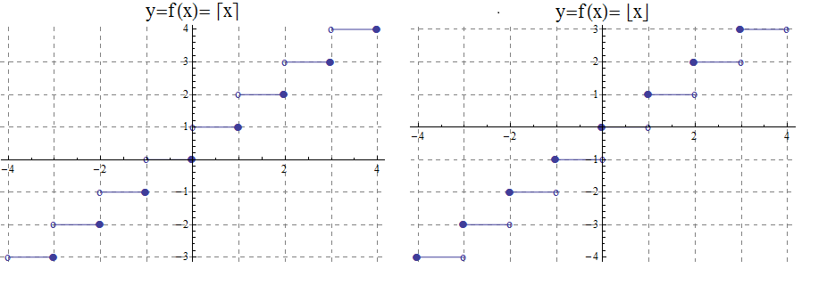
7.3.3. The Max Function
The function \(h\left(x\right)=\max{\left(f\left(x\right)\right)},\ g(x))\) is evaluated at each \(x\) for which both \(f(x)\) and \(g(x)\) are defined by the function
\( h(x) =\max(f(x),g(x)) = \left\{ \begin{array}{c} f(x) \\ g(x) \end{array} \right. \begin{array}{c} \text{if } f(x)\text{ }\geq g(x) \\ \text{if } f(x) < g(x) \end{array} \)
So for example if \(f(x) =\ \sqrt x\), and \(g(x) =x^2\) then \(h(x)=\max(f(x),g(x))\), has \(h(1/4) =\max\) \( \left(\sqrt{\frac{1}{4}},\ \left(\frac{1}{4}\right)^2\right) \) \(=max\left(\frac{1}{2},\frac{1}{16}\right)=\frac{1}{2}\), and \(h(4) =\max\) \(\left(\sqrt4,\ 4^2\right)=\max(2,16)=16\). The graph of \(h(x) =\max(\sqrt x,\ x^2)\) over the interval \((0,2)\) is shown below.
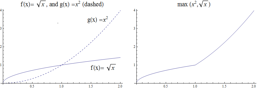
7.3.4. The Min Function
The function \(h(x) =\min(f(x),g(x))\) is evaluated at each \(x\) for which both \(f(x)\) and \(g(x)\) are defined and is similar to the \(max\) function, but is defined by the minimum of \(f(x)\), and \(g(x)\) at each \(x\).
\( h(x) =\min(f(x),g(x)) = \left\{ \begin{array}{c} f(x) \\ g(x) \end{array} \right. \begin{array}{c} \text{if } f(x)\text{ }\leq g(x) \\ \text{if } f(x) > g(x) \end{array} \)
So for example if \(f(x) =\ \sqrt x\), and \(g(x) =x^2\) then \(h(x)=\min(f(x),g(x))\), has \(h(1/4) =\min\) \( \left(\sqrt{\frac{1}{4}},\ \left(\frac{1}{4}\right)^2\right) \) \(=\min\left(\frac{1}{2},\frac{1}{16}\right)=\frac{1}{16}\), and \(h(4) =\min\) \(\left(\sqrt4,\ 4^2\right)=\min(2,16)=2\).
The graph of \(h(x) =min(\sqrt x,\ x^2)\) over the interval \([0,2 \)], is shown below
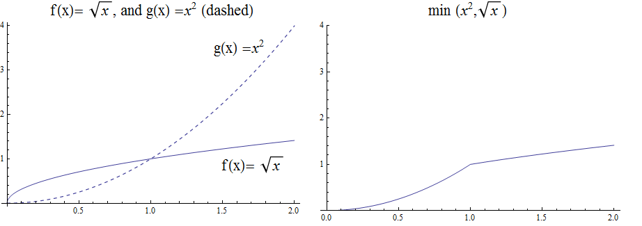
7.4. The Algebra of Functions
If two functions \(f\left(x\right)\) and \(g\left(x\right)\) have the same domain \(A\), then we can combine these functions using the common algebraic operations of addition, subtraction, multiplication, and division.
7.5. Composition of Functions
Suppose \(g:A\rightarrow B\) and \(f:B\rightarrow C\), then the functions \( f\) and \(g\), can be composed to obtain a function \(h:A\rightarrow C\), denoted as follows,
\(h\left(x\right)=\left(f\circ g\right)\left(x\right)=f\left(g\left(x\right)\right)\) provided \(x\ \in\ A\) and \(g\left(x\right)\in B\).
Notice, in the last example, that \(g\left(x\right)\) undoes \(f\left(x\right)\), in the following sense:
\(f:1\rightarrow 2\) and \(g:2\rightarrow 1\), or the ordered pair \(\left(1,2\right)\) in \(f\), corresponds to \(\left(2,1\right)\) for \(g\).
\(f:2\rightarrow 9\) and \(g:9\rightarrow 2\), or the ordered pair \(\left(2,9\right)\), in \(f\), corresponds to \(\left(9,2\right)\) for \(g\).
\(f:3\rightarrow 28\) and \(g:28\rightarrow 3\), or the ordered pair \(\left(3,28\right)\), in \(f\), corresponds to \(\left(28,3\right)\) for \(g\).
\(f:x\rightarrow x^3+1\) and \(g:x^3+1\rightarrow x\), or the ordered pair \(\left(x,x^3+1\right)\), in \(f\), corresponds to \(\left(x^3+1,x\right)\) for \(g\).
The function \$ g(x))= root(3)(x-1) \$ is said to be the inverse of the function \(f\left(x\right)=x^3+1\). We have shown explicitly that \(\left(g\circ f\right)\left(x\right)=x\).
7.6. The Inverse of a Function
In view of this relation when composing functions that are inverses of each other, we provide an intuitive definition of inverse functions.
Suppose \(f\left(a\right):A\rightarrow B\) is bijective, then the inverse of \(f\left(x\right)\), is the function denoted \(f^{-1}\left(b\right):B\rightarrow A\).
The inverse can be similarly defined for relations in general, however the bijective property is used to ensure that the inverse of a function \(f\) is also a function.
For example the following relations have inverses as given.
\(\left\{\left(-3,\ 9\right),\ \left(-2,4\right),\ \left(-1,1\right),\ \left(0,0\right),\ \left(1,\ 1\right),\ \left(2,\ 4\right),\ \left(3,9\right)\right\}\) with inverse,
\(\left \{ \left(9,-3\ \right),\ \left(4,\ -2\ \right),\ \left(1,\ -1\right),\ \left(0,0\right),\ (1,\ 1,\ \left(4,2,\right),\ (9,3)\right \}\)
Notice that the original relation can be considered a function with domain \(A=\left\{-3,\ -2,\ -1,\ 0,\ 1,\ 2,\ 3,\right\}\) and co-domain \(B=\left\{0,\ 1,\ 4,\ 9\right\}\). However the inverse mapping from domain \(A=\left\{0,\ 1,\ 4,\ 9\right\}\) with co-domain \(B=\left\{-3,\ -2,\ -1,\ 0,\ 1,\ 2,\ 3,\right\}\), is a relation that is not a function because of the mappings \(\left(-9,3\right)\), and \(\left(-9,\ 3\right)\).
7.7. Exercises
-
What can be said about the relation \(f:A\rightarrow B\), if
-
\(\exists z\in B\forall x\in A,f\left(x\right)\neq z\)
-
\(\exists x,y \in A, \exists z\in B,\left(x\neq y\right)\bigwedge\left(f\left(x\right)=f\left(y\right)=z\right)\)
-
\(\forall x,y\in A, \left(f\left(x\right)=f\left(y\right)\right)\ \rightarrow\left(x=y\right)\)
-
\(\forall x,y\in A,\left(x\neq y\right)\rightarrow\left(f\left(x\right)\neq f\left(y\right)\right)\)
-
\(\forall z\in B, \exists x,f\left(x\right)=z\)
-
\(\exists x,y\in A,\left(f\left(x\right)=f\left(y\right)\right)\bigwedge\left(x\ \neq\ y\right)\)
-
-
Explain why exponential function \(f(x)=2^x\) is not surjective from \(f: \mathbb{R} \rightarrow \mathbb{R}\), but is in fact a bijection from \(f: \mathbb{R} \rightarrow \mathbb{R}^+\).
-
Explain why ceiling function \( \left \lceil x \right \rceil\) is not surjective from \(f: \mathbb{R} \rightarrow \mathbb{R}\), but is surjective from from \(f: \mathbb{R} \rightarrow \mathbb{Z}\).
-
Use properties of logarithms to show that \(f\left(x\right)=2^x\) and \(g\left(x\right)=\log_2{x}\), where \(f, g: \mathbb{R} \rightarrow \mathbb{R}\), are inverses by verifying that \(f\left(g\left(x\right)\right)=g\left(f\left(x\right)\right)=x\).
-
Use properties of logarithms to show that \(f\left(x\right)=10^x\) and \(g\left(x\right)=\log{x}\), where \(f, g: \mathbb{R} \rightarrow \mathbb{R}\), are inverses by verifying that \(f\left(g\left(x\right)\right)=g\left(f\left(x\right)\right)=x\).
-
Show that the function \(f\left(x\right)=5x-3\), from \(f: \mathbb{R} \rightarrow \mathbb{R}\), is bijective and find its inverse.
-
Show that the function \(f\left(x\right)=2x^3-1\), from \(f: \mathbb{R} \rightarrow \mathbb{R}\) is bijective and find its inverse.
-
Consider the function \(f(x) = \left \lceil x \right \rceil\) where \(f:\mathbb{R}\rightarrow\mathbb{Z}\).
-
Is the function a surjection? Explain.
-
Is the function an injection? Explain
-
Is the function a bijection? Explain
-
Is the inverse mapping a function? Why or why not?
-
Evaluate
-
\(f\left(-2.1\right)\)
-
\(f\left(-1.9\right)\)
-
\(f\left(1.5\right)\)
-
\(f\left(1.9\right)\)
-
\(f\left(2\right)\)
-
\(f\left(2.3\right) \)
-
-
Suppose \(g\left(x\right)=2x\), with \(f\left(x\right)=\left\lceil x\right\rceil\). Evaluate the following:
-
\(f\left(g\left(2.3\right)\right)\)
-
\(g\left(f\left(2.3\right)\right)\)
-
-
-
Consider the function \(f(x) = \left \lfloor x \right \rfloor\) where \(f:\mathbb{R}\rightarrow\mathbb{Z}\).
-
Is the function a surjection? Explain.
-
Is the function an injection? Explain
-
Is the function a bijection? Explain
-
Is the inverse mapping a function? Why or why not?
-
Evaluate
-
\(f\left(-5.1\right) \)
-
\(f\left(-3.9\right)\)
-
\(f\left(-3.2\right)\)
-
\(f\left(5\right) \)_
-
\(f\left(5.3\right)\)
-
-
Suppose \(g\left(x\right)=3x\), with \(f\left(x\right)=\left\lfloor x\right\rfloor\). Evaluate the following:
-
\(f\left(g\left(5.3\right)\right)\)
-
\(g\left(f\left(5.3\right)\right)\)
-
-
-
The absolute value function, denoted \(f(x)=|x|\), where \(f\left(x\right):\mathbb{R} \rightarrow \mathbb{R}\), gives the distance from \(x\) to \(0\). For example, \(f\left(2.5\right)=\left|2.5\right|=2.5\). And \(f\left(-4.5\right)=\left|-4.5\right|=4.5\). Notice that if \(x \geq 0\), then \(\left|x\right|=x\). However if \(x<0\), then \(\left|x\right|=\ -x\). We can state this using the notation for piecewise functions:
\$f(x) = |x|={( x, if x ≥ 0),(-x,if x < 0):}\$-
Graph \(f\left(x\right)=|x|\), for -\(10\ \le x\ \le10\)
-
Evaluate
-
\(f(-5)=|-5|\),
-
\(f(-2.5)=|-2.5|\),
-
\(f(3.5)=|3.5|\).
-
-
Show that \(f\left(x\right)=\left|x\right|\), with \(f:\mathbb{R}\rightarrow \mathbb{R}\), is not injective.
-
Show that \(f\left(x\right)=\left|x\right|\), with \(f:\mathbb{R}\rightarrow \mathbb{R}\), is not surjective.
-
Consider \(g\left(x\right)=3x+2\), with \(g:\mathbb{R}\rightarrow \mathbb{R}\), and \(f\left(x\right)=|x|\). Find and simplify the following:
-
\(\left(g\circ f\right)\left(x\right)\)
-
\(\left(f\circ g\right)\left(x\right)\)
-
-
-
A real-valued function, \(f: \mathbb{R} \rightarrow \mathbb{R}\), is said to be strictly increasing if whenever \$x<y\$, then \$f(x)<f(y)\$.
-
State this using logical quantifiers.
-
State a similar definition for a strictly decreasing function, and then translate using logical quantifiers.
-
8. Growth of Functions
8.1. Introducing Big O
Computer programmers are often concerned with two questions:
a) How much time does an algorithm need to complete?
b) How much memory does an algorithm need for its computation?
Big O notation is a standard way mathematicians and computer scientists use to describe how much time and how much memory is required for an algorithm to run
Big O is typically used to analyze the worst case complexity of an algorithm. If, for example, \(n\) is the size of the input data, then Big O really only cares about what happens when your input data size \(n\) becomes arbitrarily large and not quite as interested in when the input is small. Mathematically, we want to speak of complexity in the asymptotic sense, when \(n\) is arbitrarily large. In this asymptotic sense of large \(n\), we may ignore constants. That we can ignore constants will make sense after discussing how limits, borrowed from continuous mathematics (calculus), can be used to compare the rates of growth of two different functions.
The size of the input complexities ordered from smallest to largest:
-
Constant Complexity: \(O(1)\)
-
Logarithmic Complexity: \(O(\log (n))\),
-
Radical complexity : \(O(\sqrt{n})\)
-
Linear Complexity: \(O(n)\)
-
Linearithmic Complexity: \(O(n\log (n))\),
-
Quadratic complexity: \(O(n^2)\)
-
Cubic complexity: \(O(n^3)\),
-
Exponential complexity: \(O(b^n)\), \( b > 1\)
-
Factorial complexity: \( O(n!)\)
To understand the sizes of input complexities, we will look at the graphs of functions; it is easier to consider these functions as ones that are defined for any real value input instead of just the natural numbers. This will also allow us to use continuous mathematics (that is, calculus) to analyze and compare the growth of different functions.
Radical growth is larger than logarithmic growth:
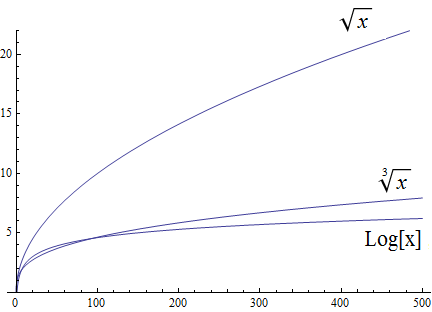
| In the preceding graph, we’ve used \(\text{Log}[x\)] to label the graph of a logarithmic function without stating the base for the logarithm: Is this the function \(y = log_{2}(x)\), \(y = log_{10}(x)\), \(y = ln(x) = log_{e}(x)\), or a logarithm to some other base? For the purposes of studying growth of functions, it does not matter which of these logarithms we use: You may recall that one of the properties of logarithms states that for two different positive constant bases \(a\) and \(b\) we must have \(log_{a}(x) = log_{a}(b) \cdot log_{b}(x)\), where \(log_{a}(b)\) is also a constant. As stated earlier, we may ignore constants when considering the growth of functions. |
Polynomial growth is larger than radical growth:
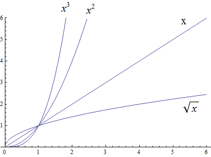
Exponential growth is larger than polynomial growth:
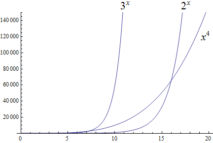
Factorial growth is larger than exponential growth:
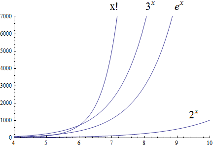
| In the preceding graph, we’ve used \(x!\) to label the graph of the function \(y = \Gamma(x+1)\) , where \(\Gamma\) is the Gamma function which is defined and continuous for all nonnegative real numbers. That is, \(n! = \Gamma(n+1)\) for every \(n \in \mathbb{N}\). Further study of the Gamma function is beyond the scope of this textbook. |
Using the graphical analysis of the growth of typical functions we have the following growth ordering, also presented graphically on a logarithmic scale graph.
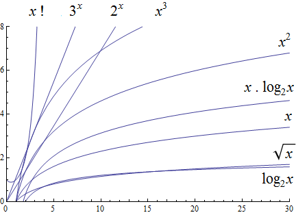
The asymptotic behavior for large \(n\) should be determined by the most dominant term in the function for large \(n\). For example, \(f(x)=x^{3} + 2x^{2}-2x\) for large \(x\), is dominated by the term \(x^3\). In this case we want to state that \(O(f(x))=x^3\). For example \(f(1000) =1.001998×10^9≈ 1×10^9 =1000^3\). For large \(x\), \(f(x) ≈x^3\) or asymptotically, \(f(x)\) behaves as \(x^3\) for large \(x\). We say \(O(f(x))=x^3\) for \(f(x)=x^3 +2x^2-2x\).
Likewise we want to say that if \(c\) is a constant that \(c \cdot f(x)\), and \(f(x)\) have the same asymptotic behavior for large \(n\), or \(O(c \cdot f(x))=O(f(x))\).
Motivated by these we formally define the Big O notation.
To determine if a function \(f(x)\) is \(O(g(x))\) amounts to identifying the positive constants \(A\) and \(n\), (sometimes called witnesses). That is, we must find the factor \( A\) and the point \( k \) for which \( f(x) \leq A g(x)\), whenever \( x > k.\)
Show that \(f\left(x\right)=2x^2 +4x\) is \(O(x^2)\)
While intuitively we may understand that the dominant term for large \(x\) is \(x^2\) so that \(f(x) = O\left(x^2\right)\), we show this formally by producing as witnesses \(A=3\) and \(n =4\) with reference to the following graph.
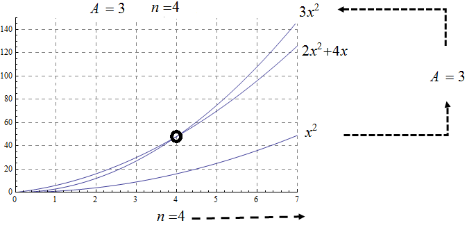
Show that \(f(x) =2x^3 +3x\) is \(O(x^3)\), with \(A=3\) and \(n=2\). Support your answer graphically.
Notice that \( x^3 > 3x\) when \( x \geq 2\). This means \(2x^3 +x^3 > 2x^3 +3x \) when \(x >2 \). In other words \( 3x^3 > 2x^3 +3x\) whenever \( x>2\), confirming \(A=3\) and \(n=2\) as witnesses, and supported by the following graph.
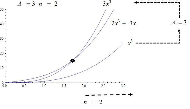
To show that a function \( f(x)\) is not \(O(g(x))\), means that no \(A\) can scale \(g(x)\) so that \( Ag(x) \geq f(x)\) for \(x\) large enough as in the following example.
Show that \( f(x) = x^2\) is not \( O( \sqrt{x})\).
Consider the graphs of \( \sqrt{x}\), \( 2 \sqrt{x}\), \( 3\sqrt{x}\), and the graph of \(x^2\). Notice that eventually, or for \(x\) large enough, \(x^2\) is larger than any \(A \sqrt{x}\) as in the figure below
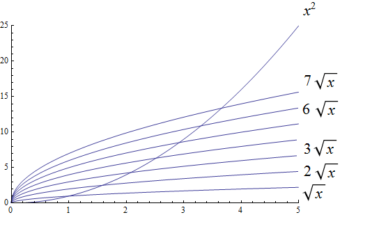
Suppose \(A>1\) is given and fixed, then if \( f(x) = x^2\) is \( O(g(x))=O( \sqrt{x})\) , there is a corresponding \(n\), also fixed, for which \(A \sqrt{x} \geq x^2\) whenever \(x>n\).
We solve the inequality \(A \sqrt{x} ≥ x^2\) by dividing both sides by \(\sqrt{x} =x^{1/2}\), to obtain, \(A \sqrt{x} ≥ x^{3/2}\).
But \(A\) is fixed and cannot be greater than all arbitrarily large \( x^{3/2}\). Hence no such \(n\) can exist for a given fixed \(A\).
For example, consider \(g(x)=A \sqrt{x}\) and \( f(x) =x^2 \), when \( x= A^2\) we obtain \( g(A^2) = A \sqrt{(A^2)}= A^2\) and \( f(A^2) = {\left ( {A}^2 \right )}^2\) and \( f(A^2)= A^4 > A^2 = g(A^2) \) when \(A>1\).
8.2. Properties of Big O notation.
Suppose \(f(x)\) is \(O(F(x))\) and \(g(x)\) is \(O(G(x))\).
We can use these properties to show for instance \( 2x^2\) is \(O\left(x^2\right)\). Likewise if \(f(x) =2x^2\) and \(g(x) =4x\), then \( 2x^2\) is \(O(x^2)\) and \( 4x\) is \(O(x)\), and the maximum gives that \(2x^2+4x\) is \( O(\max(x^2, x)) =O(x^2)\).
It is true in general that if a polynomial \(f(x)\) has degree \(n\) then \(f(x)\) is \(O(x^n)\).
For example, if \(f(x)= x^3+1\) being \( O(x^3)\), and \(g(x)=x^2-x\) being \(O(x^2)\), then \(f(x) \cdot g(x)\) is \(O(x^3 \cdot x^2) =O(x^5)\). This is verified explicitly by multiplying \(f(x) \cdot g(x)= (x^3+1) \cdot (x^2-x)= x^5 -x^4+x^2-x \) which clearly is \(O(x^5)\)
As a final example we consider ordering three functions by growth using the basic properties for Big O and the basic orderings.
8.3. Using Limits to Compare the Growth of Two Functions (CALCULUS I REQUIRED!)
In general, we have avoided using calculus methods in this textbook because calculus is part of continuous mathematics, not discrete mathematics. However, it is can be useful to use calculus to compare the growth of two functions \(f(x)\) and \(g(x)\) that are defined for real numbers \(x\), are differentiable functions on the interval \((0,\, \infty)\), and satisfy \(\lim_{x \to \infty} f(x) = \lim_{x \to \infty} g(x) = \infty\).
If \(f(x)\) and \(g(x)\) are such functions and \(\lim_{x \to \infty} \frac{f(x)}{g(x)} = L\), where \(0 \leq L < \infty\), then \(f(x)\) is \(O(g(x))\). To see this, recall that \(\lim_{x \to \infty} \frac{f(x)}{g(x)} = L\) means that we can make the value of \(\frac{f(x)}{g(x)}\) be as close to \(L\) as we want by choosing \(x\) values that are sufficiently large. In particular, we can make \(L-1 < \frac{f(x)}{g(x)} < L+1\) be true for all \(x\) greater than some real number \(r\). Now we can use the earlier stated assumption that \(0 \leq g(x)\) to rewrite the inequality as \((L-1) \cdot g(x) < f(x) < (L+1) \cdot g(x)\), which is true for all \(x > r\). We can choose for our witnesses \(A = \lceil (L + 1) \rceil\), the least integer that is greater than or equal to \(L + 1\), and \(n = \lceil r \rceil\), the least integer that is greater than or equal to \(r\). This means that \(f(x) < A \cdot g(x)\) whenever \(x > n\), which shows that \(f(x)\) is \(O(g(x))\). Note that using this method does not focus on determining the actual numerical values of \(A\) and \(n\) but just guarantees that the witnesses exist, which is all that is needed to show that \(f(x)\) is \(O(g(x))\).
8.4. Exercises
-
Give Big O estimates for
-
\(f\left(x\right)=4\)
-
\(f\left(x\right)=3x-2\)
-
\(f\left(x\right)=5x^6-4x^3+1\)
-
\(f\left(x\right)=2\ \ \sqrt x+5\)
-
\(f\left(x\right)=x^5+4^x\)
-
\(f\left(x\right)=x\log{x}+3x^2\)
-
\(f\left(x\right)=5{x^2e}^x+4x!\)
-
\(f\left(x\right)=\displaystyle \frac{x^6}{x^2+1}\) (Hint: Use long division.)
-
-
Give Big O estimates for
-
\(f\left(x\right)=2^5\)
-
\(f\left(x\right)=5x-2\)
-
\(f\left(x\right)=5x^8-4x^6+x^3\)
-
\(f\left(x\right)=\) \$4 root(3)(x)+3\$
-
\(f\left(x\right)=3^x+4^x\)
-
\(f\left(x\right)=x^2\log{x}+5x^3\)
-
\(f\left(x\right)=5{x^610}^x+4x!\)
-
\(f\left(x\right)=\displaystyle \frac{x^5+2x^4-x+2}{x+2}\) (Hint: Use long division.)
-
-
Show, using the definition, that \(f\left(x\right)=3x^2+5x\) is \(O(x^2)\) with \(A=4\) and \(n=5\). Support your answer graphically.
-
Show, using the definition, that \(f\left(x\right)=x^2+6x+2\) is \(O(x^2)\) with \(A=3\) and \(n=6\). Support your answer graphically.
-
Show, using the definition, that \(f\left(x\right)=2x^3+6x^2+3\) is \(O(x^2)\). State witnesses \(A\) and \(n\), and support your answer graphically.
-
Show, using the definition, that \(f\left(x\right)=\ {3x}^3+10x^2+1000\) is \(O(x^2)\). State the witnesses \(A\) and \(n\), and support your answer graphically.
-
Show that \(f\left(x\right)=\sqrt x\) is \(O\left(x^3\right)\), but \(g\left(x\right)=x^3\) is not\(\ O(\ \sqrt x)\).
-
Show that \(f\left(x\right)= x^2\) is \(O\left(x^3\right)\), but \(g\left(x\right)=x^3\) is not\(\ O( x^2)\).
-
Show that \(f\left(x\right)=\sqrt x\) is \(O\left(x\right)\), but \(g\left(x\right)=x\) is not\(\ O(\ \sqrt x)\).
-
Show that \(f\left(x\right)=\) \$root(3)(x)\$ is \(O\left(x^2\right)\), but \(g\left(x\right)=x^2\) is not \$O( root(3)(x))\$
-
Show that \(f\left(x\right)=\) \$root(3)(x)\$ is \(O\left(x\right)\), but \(g\left(x\right)=x\) is not \$root(3)(x)\$.
-
Order the following functions by growth \(x^\frac{7}{3},\ e^x,\ 2^x,\ x^5,\ 5x+3,\ 10x^2+5x+2,\ x^3,\log{x,\ x^3\log{x}}\)
-
Order the following functions by growth from slowest to fastest. \(\ 3x!,\ {10}^x,\ x\cdot\log{x},\ \log{x\cdot\log{x,\ \ }2x^2+5x+1,\ \pi^x,x^\frac{3}{2}\ },\ 4^5,\ \ \sqrt{x\ }\cdot\log{x}\)
-
Consider the functions \(f\left(x\right)=2^x+2x^3+e^x\log{x}\) and \(g\left(x\right)=\sqrt x+x\log{x}\). Find the best big \(O\) estimates of
-
\((f+g)(x)\)
-
\((f\cdot\ g)(x)\)
-
-
Consider the functions \(f\left(x\right)=2x+3x^3+5\log{x}\) and \(g\left(x\right)=\sqrt x+x^2\log{x}\). Find the best big \(O\) estimates of
-
\((f+g)(x)\)
-
\((f\cdot\ g)(x)\)
-
-
State the definition of "\( f(x)\) is \( O(g(x))\)"" using logical quantifiers and witnesses \(A\) and \(n\).
-
Negate the definition of "\( f(x)\) is \( O(g(x))\)" using logical quantifiers, and then state in words what it means that \( f(x)\) is not \( O(g(x))\).
9. Algorithms
COMING SOON!
10. Counting
Many of us learned how to count when we were young children, but we probably never counted up to more than 100, or perhaps at most 1000. However, there are many problems that arise in math and computer science that require counting the number of elements of sets that contain much greater numbers of elements - hundreds of thousands of elements, or millions, or even more.
This chapter introduces techniques for counting the number of elements of finite sets. These techniques can be used quickly and efficiently no matter the size of the set.
10.1. Three Basic Counting Rules
There are three basic counting rules introduced in this section, one for each of the arithmetic operations of multiplication, addition and subtraction.
10.1.1. The Product Rule (and)
To find the total number of outcomes for two or more successive events where both events must occur, multiply the number of outcomes for each event together. For instance, if you want to find the number of outcomes possible when you roll a die and toss a coin, you could use the product rule. It is important to note that the events must be independent, meaning one doesn’t effect the other.
This is called the product rule for counting because it involves multiplying to find a product. The product rule can be extended to more than two choices.
| Think of the product rule when you see AND. |
Video Example
The following video example features Dr. Joshua Roberts, Associate Professor of Mathematics at Georgia Gwinnett College.
10.1.2. The Sum Rule (xor)
Consider finding the total number of ways a particular event occurs from a variety of different mutually exclusive options (mutually exclusive means that the options do not have anything in common.) For instance, if you want to find the number of ways to pick, at random, a student enrolled in Discrete Math this semester, you could use the sum rule to add the number of students in each section of Discrete Math (assuming that no student is enrolled in more than one section).
This is called the sum rule for counting because it involves adding to find a total. The sum rule can also be extended to more than two choices.
| Think of the sum rule when you see OR. |
Video Example
The following video example features Dr. Katherine Pinzon, Professor of Mathematics at Georgia Gwinnett College.
10.1.3. The Subtraction Rule (or)
If your events are not mutually exclusive, to find the total number of possibilities use the subtraction rule.
Video Example
10.2. The Pigeonhole Principle
A suprising number of counting problems can be solved with the so-called pigeonhole principle.
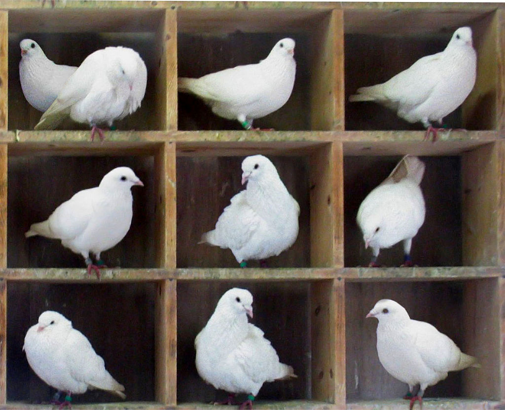
Ten pigeons in nine pigeonholes
10.3. Permutations and Combinations
Many counting problems involve choosing, from a set of \(n\) objects, either an ordered sequence of \(r\) objects or a subset of \(r\) objects, with no repetition allowed. We will describe ways to do this type of counting in this section.
10.3.1. Permutations
A permutation of a set of elements is an ordered arrangement of the elements. A permutation may involve every element of the set, or only some of the elements of the set.
Consider the first four letters of the English alphabet, \(A, B, C, D\).
-
\(ABCD, BACD, ABDC\) are permutations of the letters taken four at a time
-
\(BDA, ABC, ABD\) are permutations of the letters taken three at a time
-
\(AB, AC, DB\) are permutations of the letters taken two at a time
By listing all possible permutations of \(A, B, C, D\), we can determine that there are 24 permutations of the letters taken four at a time, 24 permutations of the letters taken three at a time, and 6 permutations of the letters taken three at a time. But what if we wanted to find all the possible permutations of the twenty six letters \(A, B, C, D, \ldots , X, Y, Z\)? It is very time consuming to write out all possible permutations of the twenty six letters taken, say, twenty one at a time, so we will develop a method and formula for doing this.
In general, given a set of \(n\) objects, an ordered arrangment of \(r \le n\) of the objects is called an \(r\)-permutation or a permutation of \(n\) objects taken \(r\) at a time. We use the notation \(P(n,r)\) to represent the number of permutations of \(n\) objects taken \(r\) at a time. Note that \(_nP_r\) is another commonly used notation, especially on calculators.
Suppose we have \(n\) objects and want to construct a \(2\)-permutation of the objects. There are \(n\) possible choices for the first object, and once that object is chosen, there are \(n-1\) possible choices for the second object. We now use the product rule to conclude that there are \(n(n-1)\) ways to choose the two objects; note that the order of the choices matters here.
We can generalize this argument, informally, as follows: Suppose we have \(n\) objects and want to construct an \(r\)-permutation, where \(r \le n.\) There are \(n\) possible choices for the first object, \(n-1\) possible choices for the second object, and so on, until we have \(n-(r-1)\) possible choices for the \(r\text{th}\) object. Apply the product rule repeatedly to find that there are \( n(n-1)\cdots (n-r+1)\) \(r\)-permutations of the \(n\) objects.
Note that a formal proof can be done by using mathematical induction.
The previous code example gives evidence for the following theorem. Again, a formal proof can be done by using mathematical induction.
Video Example
10.3.2. Combinations
A selection of objects from a set of \(n\) objects where order of selection does not matter is called a combination. Notice that each combination corresponds to a subset of the set of \(n\) objects.
Consider the letters \(A, B, C, D\) and choose three at a time where the order does not matter. In this case we are selecting a subset of size three instead of a sequence of length three. The sets \(\{ A, B, C \}\) and \(\{ B, C, A \}\) are just two ways of describing the same set since the order in which elements of a set are listed does not matter.
-
There are four possible ways to choose three letters without regard to order: \(\{ A, B, C \}\), \(\{ A, B, D \}\), \(\{ A, C, D \}\), and \(\{ B, C, D \}\).
-
There are six possible ways to choose three letters without regard to order: \(\{ A, B \}\), \(\{ A, C \}\), \(\{ A, D \}\), \(\{ B, C \}\), \(\{ B, D \}\), and \(\{ C, D \}\).
-
There are four possible ways to choose one letter (without regard to order): \(\{ D \}\), \(\{ C \}\), \(\{ B \}\), and \(\{ A \}\). (Keep reading to find out why this "reversed" ordering of the subsets was used.)
This shows that there are 4 combinations of 4 objects taken 3 at a time, 6 combinations of 4 objects taken 2 at a time, and 4 combinations of 4 objects taken 1 at a time.
In general, given a set of \(n\) objects, an unordered selection of \(r\le n\) of them is called an \(r\)-combination or a combination of \(n\) objects taken \(r\) at a time. We will denote this by \(C(n,r)\), read as '\(n\) choose \(r\)'. Note that \(_nC_r\) is commonly used by calculators.
Using this notation, we can write \(C(4,3) = 4\), \(C(4,2) = 6\), and \(C(4,1) = 4\).
Notice that \(C(4,3) = C(4,1)\); it may appear that this "just happens to be true", but in fact is an example of the next theorem. In this case, a combination of 4 objects taken 3 at a time corresponds to a combination of 4 objects taken 1 at a time - we can choose 3 of the 4 elements by "throwing out" the 1 element we don’t want to keep. That is, we choose the 3-element subset we care about indirectly by instead choosing the 1-element complement of the subset.
In general, there is always a one-to-one correspondence between the combinations of \(n\) objects taken \(r\) at a time and the combinations of \(n\) objects taken \(n-r\) at a time: Choosing \(r\) elements for a subset corresponds to choosing the \(n-r\) elements for the complement of the subset.
A formal proof of the theorem can be written by proving that, for any set \(S\), the function with domain and codomain \(\mathcal{P}(S)\) and that maps each subset of \(S\) to its complement is both injective and surjective.
Next, notice that every \(r\)-combination corresponds to \(P(r, r) = r!\) different \(r\)-permutations. That is, to select a \(r\)-permutation we could instead first select a \(r\)-combination without regard to order and then order the \(r\) elements.
As an example, suppose we have \(n\) objects and want to construct a \(3\)-permutation. We could instead first choose a \(3\)-combination of the objects. There are \(C(n,3)\) possible \(3\)-combinations. Once we have chosen a specific \(3\)-combination, we can reorder the 3 elements in \(P(3,3) = 3!\) ways. This argument shows that \(P(n,3) = C(n,3) \cdot P(3,3) = C(n,3) \cdot 3!\), so \(C(n,3) = \displaystyle \frac{P(n,3)}{3!}\).
We can generalize this argument for each natural number \(r \leq n\) to arrive at the next theoren.
A formal proof of the theorem can be done by using mathematical induction.
Video Example
Video Example
10.4. Exercises
-
There are 67 math majors and 124 ITEC majors at a college.
-
In how many ways can two representatives be picked so that one is a math major and one is an ITEC major?
-
In how many ways can one representative be picked who is either a math major or an ITEC major?
-
-
A multiple-choice test contains 20 questions, and each question has four choices.
-
In how many ways can a student answer all of the questions on the test?
-
In how many ways can a student answer all of the questions if she is allowed to leave some blank?
-
-
How many different three-letter initials can a person have?
-
How many different three-letter initials end with "R"?
-
How many bit strings are there of length five?
-
How many bit strings are there of length five that begin and end with 1?
-
How many bit strings are there of length less than \(n\), where \(n\) is a positive integer, that start and end with 1?
-
How many license plates can be made using three digits followed by four uppercase English letters if:
-
Digits and letters can be repeated?
-
Digits and letters cannot be repeated?
-
-
If each student in Discrete Mathematics is a mathematics major, an ITEC major, or a double major, and a class has 5 math majors (including double majors), 23 ITEC majors (including double majors), and 7 double majors, how many students are in the class?
-
Suppose a computer system requires a password of length no less than 7 and no more than 10 characters, and each character must be an English lowercase letter, an English uppercase letter, a digit, or one of six special characters (*, >, <, !, +, =).
-
How many different passwords are available?
-
Suppose a hacker can check a potential password once every nanosecond (1 nanosecond is \(1 \times 10^{-9}\) seconds). How long will it take the hacker to check every potential password?
-
-
Show that if there are 29 students in a class at least two have last names that begin with the same letter.
-
How many students need to be in a class in order for at least two students to receive the same grade on an exam that is graded on a scale 0 to 100 points?
-
Show that in any set of 5 integers, there are at least two of them that have the same remainder when divided by 4.
-
A bag contains 8 red balls and 7 blue balls.
-
How many balls must be chosen to be sure of choosing 3 of the same color?
-
How many must be chosen to be sure of choosing 3 red balls?
-
-
Someone cleaning out their attic finds a box containing 12 rock CDs and 12 country CDs. What is the minimum number of CDs they can take out to guarantee at least one of each type?
-
Give an argument that there are at least two people in Atlanta with the same number of hairs on their head.
-
There are 67 math majors and 124 ITEC majors at a college.
-
In how many ways can two representatives be picked so that one is a math major and one is an ITEC major?
-
In how many ways can one representative be picked who is either a math major or an ITEC major?
-
-
A multiple-choice test contains 20 questions, and each question has four choices.
-
In how many ways can a student answer all of the questions on the test?
-
In how many ways can a student answer all of the questions if she is allowed to leave some blank?
-
-
How many different three-letter initials can a person have?
-
How many different three-letter initials end with "R"?
-
How many bit strings are there of length five?
-
How many bit strings are there of length seven that begin and end with 0?
-
How many bit strings are there of length less than \(n\), where \(n\) is a positive integer, that start and end with 1?
-
How many license plates can be made using four digits followed by three uppercase English letters if:
-
Digits and letters can be repeated?
-
Digits and letters cannot be repeated?
-
-
If each student in Discrete Mathematics is a mathematics major, an ITEC major, or a double major, and a class has 18 math majors (including double majors), 25 ITEC majors (including double majors), and 8 double majors, how many students are in the class?
-
Suppose a computer system requires a password of length no less than 8 and no more than 11 characters, and each character must be an English lowercase letter, an English uppercase letter, a digit, or one of six special characters (*, >, <, !, +, =).
-
How many different passwords are available?
-
Suppose a hacker can check a potential password once every nanosecond (1 nanosecond is \(1 \times 10^{-9}\) seconds). How long will it take the hacker to check every potential password?
-
-
Show that if there are 29 students in a class at least two have last names that begin with the same letter.
-
How many students need to be in a class in order for at least two students to receive the same grade on an exam that is graded on a scale 0 to 50 points?
-
Show that in any set of 8 integers, there are at least two of them that have the same remainder when divided by 7.
-
A bag contains 12 red balls and 7 blue balls.
-
How many balls must be chosen to be sure of choosing 4 of the same color?
-
How many must be chosen to be sure of choosing 4 red balls?
-
-
Someone cleaning out their attic finds a box containing 12 rock CDs, 12 hip hop CDs, and 12 country CDs. What is the minimum number of CDs they can take out to guarantee at least one of each type?
-
Give an argument that there are at least two people in Atlanta with the same number of hairs on their head.
-
List all the permutations of \(\{1, 2, 3\}\).
-
How many permutations are there of the set \(\{1, a, 2, b, 3, c, 5\}\)?
-
Let \(A=\{a, b, c, d\}\)
-
List all the 3-permutations of \(A\).
-
List all the 3-combinations of \(A\).
-
-
Let \(A=\{a, b, c, d, e\}\)
-
List all the 2-permutations of \(A\).
-
List all the 2-combinations of \(A\).
-
-
Find the value of the following
-
\(P(5,2)\)
-
\(P(10,8)\)
-
\(P(14,10)\)
-
\(P(12,8)\)
-
\(C(5,2)\)
-
\(C(10,8)\)
-
\(C(14,10)\)
-
\(C(12,8)\)
-
-
How many bit strings of length 10 contain:
-
Exactly five 1s?
-
At most five 1s?
-
At least four 1s?
-
The same number of 0s and 1s?
-
-
How many permutations of the digits \(12345678\) contain:
-
The string 284?
-
The string 3581?
-
The string 21 and 57?
-
-
How many ways are there to choose 9 cards from a standard 52 card deck?
-
How many ways can you be dealt a pair in a 5 card hand (2 cards of the same rank and 3 cards of a different rank)?
-
How many ways can you be dealt a full house in a 5 card hand (2 cards of the same rank and 3 cards of the same rank)?
-
How many license plates consist of 4 letters followed by 3 digits if:
-
Repetition is allowed?
-
Repetition is not allowed?
-
-
Using \(C(n,r) = \displaystyle \frac{n!}{r!(n-r)!}\), evaluate the terms of this triangular table. Will you need the formula to extend the table to more rows?
\begin{array}{ccccccccccccc} &&&&&&&C(0,0)&&&&&&\\ &&&&&& C(1,0) && C(1,1) &&&&&\\ &&&&& C(2,0) && C(2,1) && C(2,2) &&&&\\ &&&& C(3,0) && C(3,1) && C(3,2) && C(3,3) &&&\\ &&& C(4,0) && C(4,1) && C(4,2) && C(4,3) && C(4,4) &&\\ \end{array}
11. Number Theory
COMING SOON!
12. Sequences and Recursive Definitions
COMING SOON!
13. Graph Theory
Graphs are discrete mathematical structures that have many applications in a diversity of fields including chemistry, network analysis, algorithms, and social sciences.
13.1. Introduction and Basic Definitions
A graph consists of a set of vertices (also called nodes) and a set of edges, where each edge either connects two different vertices or connects a vertex to itself.
-
For each edge, its endpoints are the vertices that it connects. The edge is said to be incident with each endpoint, and to connect the endpoints.
-
If an edge has only one endpoint, it is called a loop.
-
An isolated vertex is a vertex that is not an endpoint of any edge.
-
If two or more edges connect the same endpoints (or endpoint if the edges are loops), the graph is called a multigraph.
-
A simple graph is a graph that has no loops and does not have two or more edges that connect the same endpoints.
Graphs discussed in this textbook are assumed to be simple unless stated otherwise.
The graph shown has 7 vertices and 7 edges.
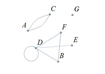
This is one graph that is made up of three separate connected components (Connectivity will be defined in detail later in the chapter, but is introduced informally here).
-
One connected component contains the vertices \(A\) and \(C\) and two edges that connect them.
-
A second connected component contains the vertices \(B\), \(D\), \(E\), and \(F\) and the edges that are incident to those vertices.
-
A third connected component contains the single isolated vertex \(G\) and no edges.
In the second connected component, the graph is drawn so that the edge with endpoints \(B\) and \(F\) and the edge with endpoints \(D\) and \(E\) cross, but the point of intersection is ignored because it is not a vertex. We could redraw this graph so that the two edges do not cross; for example, we could move \(E\) inside the triangle. However, there are some graphs which cannot be drawn in 2 dimensions without some edge crossings.
This graph is a multigraph because there are multiple edges that connect the pair of vertices \(\{A,C\}\).
This graph is not simple because (1) it contains a loop and (2) it has a pair of vertices that are connected by two different edges.
MORE TO COME!
14. Appendix 0: An Introduction to Python
14.1. Programming Basics
Computers are programmable machines that process information by manipulating data. As the data can represent any real world information, and programs can be readily changed, computers are capable of solving many kinds of problems.
14.1.1. Programming Languages and Environments
There are many different programming languages for programmers to choose from. Each language has its own advantages and disadvantages, and new languages gain popularity while older ones slowly lose ground. In this book, we use the Python 3 programming language. It is popular in both academia and industry, and was designed with education in mind.
14.1.2. PythonTutor
PythonTutor is an environment for creating very short and simple Python programs and visualizing their execution. This enables beginners to visually see the data as it gets manipulated by the instructions.
14.1.3. Comments
Program files can contain source code and comments. Comments are not instructions for the computer to follow, but instead notes for programmers to read. Comments in Python start with a pound sign (#). Anything following the pound sign that is on the same line as the pound sign will not be executed. Often, at the very beginning of a program, comments are used to indicate the author and other information. Comments are also used to explain tricky sections of code or disable code from executing.
# This line is not Python code, it is a comment.

score = 9001 # over 9000!!!

# The next line of code is disabled because is starts with a #.
# score = 8000
14.2. Data Types
Programming is all about information processing. Information is categorized by data types. Four basic data types we will be considering are int, float, bool, and str. Int consists of integers, which are whole numbers written without a decimal point. This includes positive and negative whole numbers as well as zero. Float consists of floating-point numbers, which are numbers that are written with a decimal point. Bool consists of Boolean values (named after the mathematician George Boole). The only Boolean values are True and False. Str consists of strings, which are sequences of text characters including punctuation, symbols, and whitespace. Every value in Python has a corresponding data type. The table below shows examples of ints, floats, and strings.
| Data Type | Example Values |
|---|---|
int |
2, -2, 0, 834529 |
float |
3.14, -2.3333, 7.0 |
bool |
True, False |
str |
"Hello World!", 'Coconut', "0", '4 + 6' |
|
Strings and Quotation Marks
Strings are always surrounded by quotation marks. Python allows either single (') or double (") quotation marks. Some strings may look like numbers, but as long as they are surrounded by quotation marks, they are treated like text. |
14.3. Variables
Variables are (virtual) boxes that store values for reuse later. A variable has a name and a current value. Each variable can only hold one value at a time. Variables are assigned a value using the single equal sign (=). As Python executes one line at a time, variables come into existence on the line where they are first assigned. Each variable only stores the most recent value assigned to it.
|
Variable Names
Variables can have complex names like player1_score. In general, never start a variable name with a number and never use spaces in variable names. |
14.4. Operators and Expressions
|
Expression Evaluation
When Python encounters a line with an expression, it always evaluates the expression first. Consider the following line of code: Python first calculates the value of the expression to the right of the equal sign by using the standard order of operations starting inside the parentheses. The value given by the above expression is calculated to be equal to 14. Then, Python creates the variable x and assigns the value 14 to this variable. The variable only stores the calculated value, not the entire expression that generated that value. |
14.5. Strings and Printing
Besides creating and storing values in variables, we can also output text on a screen by calling the print() function.
14.6. If Statements
A block of code is a collection of lines of code that are either all executed (in sequential order) or all skipped. Blocks always start with a colon (:) on the previous line and require every line in the block to be indented the same amount using tabs or spaces. One way in which Python can execute or skip over a block involves using an if command and a Boolean expression. If the expression is true, then the block executes. Othewise, the block is skipped.
When you want to force exactly 1 of 2 blocks to execute (as opposed to just skipping a block), you can use the else command in addition to the if command. If the expression following the if command is true, then the first block executes. Otherwise, the second block executes.
In order to force exactly 1 of more than 2 blocks to execute, you can use the elif command in addition to the if and else commands. Each elif command must be followed by a Boolean expression. When using if and elif commands, each expression is checked in sequential order, and the block following the first true expression executes. If none of the expressions are true, the block following the else command is executed.
14.7. While Statements
Python can execute a block repeatedly using a while statement and a Boolean expression. The block repeats until the Boolean expression is false.
| The += operator increases the value of the variable written to the left of the operator by the value written to the right of the operator. |
14.8. Lists and Loops
When you need to consider many values at once, use a list.
When you want to consider every value in a list, use a for loop.
| The range() function returns a sequence of numbers. The sequence starts at the value given by the first argument, increments by 1, and ends at one less than the value given by the second argument. For example, range(2,5) returns 2,3,4. If only one argument is given, that argument is considered the second argument and the first argument is set to 0 by default. For example, range(4) returns 0,1,2,3. |
14.9. List Appending and Slicing
We can append to lists with the concatenation operator (+). We can also slice a list using the bracket notation and two indices separated by a colon (:). The first index specifies the starting point of the slice while the second index specifies the stopping point of the slice + 1.
14.10. Defining Custom Functions
In the examples above we have called several functions like print() and len(). You can define your own functions using def. A function definition includes zero or more parameter variables. The values of those parameter variables are referred to as the arguments of the function.
14.11. Exercises
-
Given the following Python code, what is the value and data type of each variable?
a = 6 + 8 large = a // 4 b = 22 // 3 c = 22 % 3 d = False or True e = True and False sheep = (True or (b > 10)) -
Given the following Python code, determine the printed output.
print("Hello World!") a = "The answer is" b = 6 * 7 print(a, b) print(False, "Hobbit", 1, "Ring") -
For the following code, determine the value of the variable letter when the score is 92, 84 and 59.
score = #an interger between 0 and 100 if score >= 90: letter = 'A' elif score >= 80: letter = 'B' elif score >= 70: letter = 'C' elif score >= 60: letter = 'D' else: letter = 'F' -
For the following code, determine the value of the variable ans for each case given below.
if outside == False: if (n >= 2 and n <= 20): return ans = True else: return ans = False else: if (n <= 2 or n >= 20): return ans = True else: return ans = False-
n = 3, outside = False
-
n = 15, outside = False
-
n = 15, outside = True
-
n = 12, outside = True
-
-
What will this code print out?
while count > 0: print("Welcome") count -= 1 -
Write Python code to satisfy the following conditions. Then test your code on the values of the variables given.
-
Given an int n, return the absolute diffrence between n and 10, except return triple the absolute dfference if n is over 10. It should return 1 when n=9. It should return 33 when n=21. What will the code return when n=7 or n=35?
-
We have a loud talking robot. The "hour" parameter is the current hour time in the range 0 to 23. We are in trouble if the robot is talking and the hour is before 6 or after 21. Return True if we are in trouble. It should return True when the robot is talking and the hour is 8. It should return False when the robot is not talking and the hour is 8. What does it return if the robot is talking and the hour is 9?
-
-
What will the following code print out?
numbers = [1, 3, 5, 7, 10] sq = 0 for val in numbers: sq = val * val print(sq) -
What will the following code print out?
for i in range(1, 20, 2): print(i) -
Use the following definition of the function front3() to find the output of the program for the list [1, 3, 5, 7].
def front3(nums): i = 0 while (i < len(nums) and i < 5): if nums[i] == 3: return True i += 1 return False -
Write a function that takes, as input, two lists of integers, a and b, both of length 3, and returns, as output, a new list of length 2 containing the last elements of a and b. For example, if a = [1, 2, 3] and b = [10, 20, 30], then the function should return the list [3, 30].
15. Appendix 1: Library of Functions
Functions can in many cases be visualized graphically, for example when mapping from the real line, \(\mathbb{R}\) to the real line, such maps are viewed on a Cartesian plan.
15.1. Quadratic Function
The function \(f(x) =x^2\), denotes the association \((a,b) =(x, x^2)\) with \(f : \mathbb{R} \rightarrow \mathbb{R}\). We notice that the range is the set of real numbers \([0, \infty)= \mathbb{R}^{+}\). The function is not invertible, since it is not injective. For example, we have both \(f(-3) =9\) and \(f(3)=9\). With \(f : \mathbb{Z} \rightarrow \mathbb{Z}\) notice that the range is now \(\mathbb{N}\)
\begin{array}{lccccccccccc} & x & -5 & -4 & -3 & -2 & -1 & 0 & 1 & 2 & 3 & 4 & 5 \\ & x^2 & 25 & 16 & 9 & 4 & 1 & 0 & 1 & 4 & 9 & 16 & 25 \end{array}
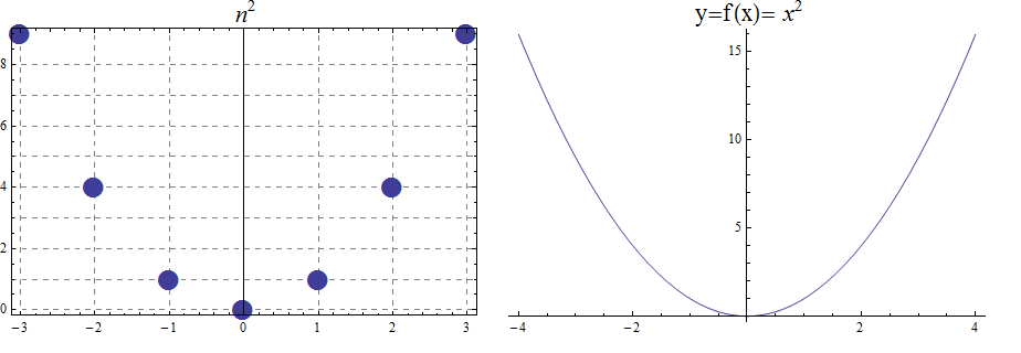
15.2. The Cubic function
The function \(f(x) =x^3\), denotes the association \((a,b) =(x, x^3)\) with \(f : \mathbb{R} \rightarrow \mathbb{R}\). Also, we notice that the range is the set of all real numbers \((- \infty , \infty)=\mathbb{R}\). The function is bijective and so invertible. With \(f : \mathbb{Z} \rightarrow \mathbb{Z}\), notice that the range, in addition to domain, is also \(\mathbb{Z}\)
\begin{array}{llcccccccccl} & x & -5 & -4 & -3 & -2 & -1 & 0 & 1 & 2 & 3 & 4 & 5 \\ & x^3 & -125 & -64 & -27 & -8 & -1 & 0 & 1 & 8 & 27 & 64 & 125 \end{array}
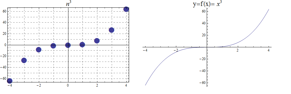
15.3. The Square Root and Cube Root Functions
For the purposes of completeness and for comparing how fast functions \(f(x)\) grow for large x, we present the inverse of the functions \(f(x)= x^2\) and \(f(x)= x^3\), when \(f(x):\mathbb{R}+→\mathbb{R}+\). Respectively, the functions\( f(x)=\sqrt{x}\) and \(f(x)= \) \$root(3)(x)\$.
\begin{array}{lcccccccccclll} & x & 0 & 1 & 4 & 9 & 16 & 25 & 36 & 49 & 64 & 81 & 100 & 121 & 144 \\ & \sqrt{x} & 0 & 1 & 2 & 3 & 4 & 5 & 6 & 7 & 8 & 9 & 10 & 11 & 12 \end{array}
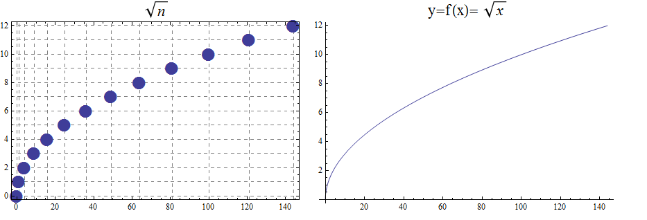
\begin{array}{lcccccl} & x & 0 & 1 & 8 & 27 & 64 & 125 \\ & \sqrt[3]{x} & 0 & 1 & 2 & 3 & 4 & 5 \end{array}
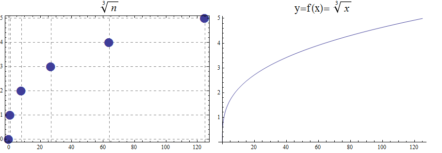
15.4. Exponential and Logarithmic Functions
We begin by summarizing important properties of exponentials.
15.4.1. Exponential Functions
Exponential functions are of the form \(f\left(x\right)=b^x\), where \(b\) is the base and the variable \(x\) is in the exponent. The base \(b>0\) and \(b ≠ 1\). Properties of exponential functions come from properties of exponents. When the base \(b\) is greater than 1 the exponential function is increasing exponentially, as in the case \(f(x) = 2^x\).
\begin{array}{llcccccccccl} & x & -5 & -4 & -3 & -2 & -1 & 0 & 1 & 2 & 3 & 4 & 5 \\ & 2^x & \frac{1}{32} & \frac{1}{16} & \frac{1}{8} & \frac{1}{4} & \frac{1}{2} & 1 & 2 & 4 & 8 & 16 & 32 \end{array}
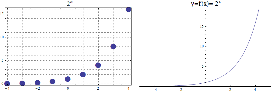
When the base \(b\) is less than 1 the exponential function is decreasing exponentially, as in the case \(f(x) = \left(\frac{1}{3}\right) ^x\).
\begin{array}{llcccccccccl} & x & -5 & -4 & -3 & -2 & -1 & 0 & 1 & 2 & 3 & 4 & 5 \\ & (\frac{1}{3})^x & 243 & 81 & 27 & 9 & 3 & 1 & \frac{1}{3} & \frac{1}{9} & \frac{1}{27} & \frac{1}{81} & \frac{1}{243} \end{array}
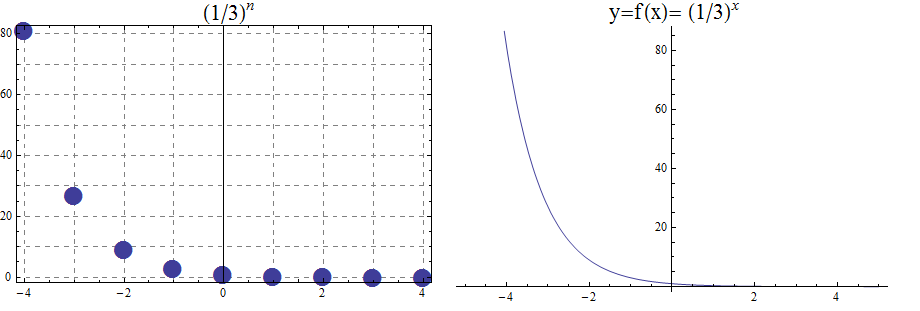
15.4.2. Logarithmic Functions
Logarithmic functions are the inverse functions corresponding to exponential functions and are used to solve exponential equations. For example, \(y=2^x\) is solved for \(x\) by inverting \(x=\log_2{y}\). Properties of logarithms follow from this relationship between exponentials and logarithms and properties of the exponentials.
We summarize three important properties of logarithms.
All other properties of logarithmic functions come from properties relating the logarithm as the inverse of the exponential and the equivalence of the logarithm \(a =\log_b m\) with \(b^a=m\).
When the base \(b\) is greater than 1, the logarithm function is increasing, as in the case \(f(x) = \log_2 x\).
\begin{array}{llllllcccccc} & x & \frac{1}{32} & \frac{1}{16} & \frac{1}{8} & \frac{1}{4} & \frac{1}{2} & 1 & 2 & 4 & 8 & 16 & 32 \\ & log_2 x & -5 & -4 & -3 & -2 & -1 & 0 & 1 & 2 & 3 & 4 & 5 \end{array}
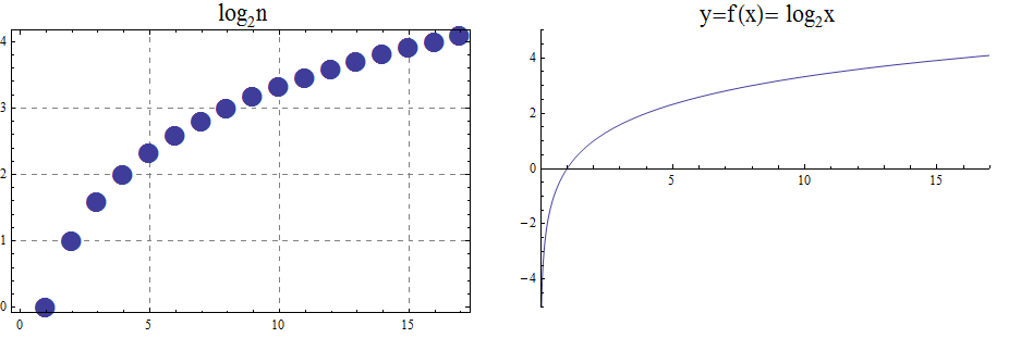
When the base \(b\) is less than 1, the logarithm function is decreasing exponentially, as in the case \(f(x) = \log_{\frac{1}{3}} \ x\).
\begin{array}{llllllcccccl} & x & \frac{1}{243} & \frac{1}{81} & \frac{1}{27} & \frac{1}{9} & \frac{1}{3} & 1 & 3 & 9 & 27 & 81 & 243 \\ & \log_{\frac{1}{3}} x & 5 & 4 & 3 & 2 & 1 & 0 & -1 & -2 & -3 & -4 & -5 \end{array}
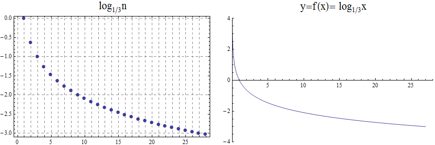
16. Appendix 2: Python Syntax Examples
1
2
3
4
5
6
7
8
9
10
11
12
13
14
15
16
17
18
19
20
21
22
23
24
25
26
27
28
29
30
31
32
33
34
35
36
37
38
39
40
41
42
43
44
45
46
47
48
49
50
51
52
53
54
55
56
57
58
59
60
61
62
63
64
65
66
67
68
69
70 # the '#' character makes a COMMENT separating Python from English
x = 3 # create the VARIABLE with NAME x and STORE INT VALUE 3
Sebastien_Score = 9001 # variable names can be long, but no spaces!
y = 1.0 * 3 # y stores EXPRESSION's RETURN FLOAT value 3.0
z = "Hi There!" # z stores a STRING value
w = False # w stores a BOOLEAN value
v = [3, 30, "Hello World"] # v stores a LIST of values
print(z) # print function displays output ("Hi There!")
# Maths
a = 3
b = 3.0 # b stores 3.0 (float values are decimal approximations)
c = 7 // 2 # c stores 3 (int division always gives ints)
d = 7 % 2 # d stores 1 (Mod or Remainder of the division)
a = 5 # change the value of a to 5
a += 1 # INCREMENT the value of a by 1 (to 6)
# Boolean Operators
a = (3 > 2) # a stores True because 3 is greater than 2
a = (2 >= 2) # a stores True because 2 is greater than or equal to 2
a = (3 < 2) # a stores False because 3 is not less than 2
a = (2 <= 2) # a stores True because 2 is less than or equal to 2
a = (3 != 2) # a stores True because 3 is not equal to 2
a = (3 == 3) # a stores True because 3 is equal to 3
a = (True and False) # a stores False, AND returns True only when both sides are True
a = (True or False) # a stores True, OR returns True if at least 1 side is True
a = (not False) # a stores True, NOT returns opposite
# BLOCKS are sections of any code chunked together with INDENTATION
# BLOCKS start with a ':' and continue with each INDENTED line
x = 7
if x > 8: # if CONDITION is True, then execute block, otherwise skip block.
print("Hello") # since x stores 7, this will skip
print("I Am Sam.") # since x stores 7, this will skip
elif x > 2: # elif condition is True AND previous if was False, execute block
print("Hi") # since x stores 7, this will execute
print("I am Sally.") # since x stores 7, this will execute
else: # if all previous conditions are False, executer block.
print("Yo") # since x stores 7, this will skip
print("I'm Bob.") # since x stores 7, this will skip
while x > 3: # repeat a block until condition becomes False
print("Apples")
x += -1
# Lists store multiple values
a = [10, 30, 20, 90] # create a new list
x = len(a) # x stores 4 (the length)
b = a[0] # INDEX into the list, 0 is first value, b stores 10
c = a[3] # c stores 90
d = a[-1] # -1 is last value, d stores 90
e = a[1:3] # slice a from index 1 up to index 3, e stores [30, 20]
a[1] = 50 # modify the second element in the list, a is now [10, 50, 20, 90]
f = a + [5, 15] # f stores [10, 50, 20, 90, 5, 15], CONCATENATION not addition
g = range(0, 4) # range function returns list 0 up to 4, g stores [0, 1, 2, 3]
# For Loops
for c in "Elephant!": # repeat block with c storing each character 1 at a time
print(c) # prints one letter per line
for x in [10, 30, 20]:
print(x) # prints one number per line
# Custom Functions
def myfunc(a, b): # DEFINES a new function that takes 2 INPUT PARAMETER values
c = 2 * a + b # executes only when function is called
return c # RETURNS a value back to the calling code
x = myfunc(10, 5) # Calls the myfunc() function, x stores return value 25
y = myfunc(1, 3) # Calls the myfunc() function, x stores return value 5
17. Appendix 3: Just-In-Time Math Review
17.1. Linear Functions And Their Equations
A linear function is one that has a constant rate of change.
\begin{array}{|l|c|c|c|c|c|} & x & 1 & 2 & 3 & 4 & 5 \\ \hline \\ & y & 1 & 3 & 5 & 7 & 9 \end{array}
The table above displays a function with independent variable \(x\) and dependent variable \(y\).
Notice that the value of \(y\) increases by \(2\) for each increase in \(x\) by \(1\). The rate of change of this function is \(2\); this corresponds to the slope \(m\) of the continuous line that passes through the points with \(xy\)-coordinates given in the table.
The vertical intercept \(b\) (in this case, the \(y\)-intercept) is the \(y\)-value that corresponds to \(x = 0\), that is, \((0,\,b)\) is on the same continuous line as the points represented in the table. In this example, \(0\) is not a value of \(x\), but we can still find the vertical intercept by subtracting \(1\) from the smallest \(x\)-value and subtracting \(2\) from the corresponding \(y\)-value , which tells us that the point \((0,\,-1)\) lies on the same continuous line as the points represented in the table.
The equation of the linear function determined by the points in the table is \(y = 2 \cdot x + (-1)\), which can be written more simply as \(y = 2x - 1\). This also is the equation of the continuous line that passes through the points with \(xy\)-coordinates given in the table, but the linear function can be restricted to a smaller domain as needed by the context where it is being used, for example, we may only need to use inputs \(x\) from the set of positive integers or possibly just the set \(\{ 1,\,2,\,3,\,4,\,5 \}\).
MORE TO COME!