14. Graphs
CAUTION - CHAPTER UNDER CONSTRUCTION!
NOTICE: If you are NOT enrolled in the CSC 230 course that I teach at SFSU, you probably are looking for the “public version” of the book, which I only update between semesters. The version you are looking at now is the “CSC230 version” of the book, which I will be updating throughout the semester.
This chapter was last updated on November 29, 2025.
Added content to subsection on the Traveling Salesperson Problem.
Revised example involving isomophism and planarity.
Revised and expanded the discussion of isomorphisms and underlying graphs.
Graphs are discrete mathematical structures used to represent connections between individual Graphs have applications in fields such as chemistry, network analysis, computing algorithms, and social sciences.
Key terms and concepts covered in this chapter:
-
Graphs
-
Undirected graphs
-
Directed graphs
-
Weighted graphs
-
-
Creating new graphs from old graphs
-
Subgraphs
-
Unions and intersections of graphs
-
-
Graph isomorphism
-
Graph coloring
-
Connectivity of graphs
-
Eulerian circuits
-
Hamiltonian circuits
-
Shortest-path problems
-
Dijkstra’s algorithm
-
Traveling Salesperson Problem (TSP)
-
-
14.1. Introduction and Definitions
A graph consists of a set of vertices and a set of edges. Each edge connects either two different vertices or one vertex to itself. Vertices are sometimes called nodes.
-
For each edge, its endpoints are the two vertices that it connects (but notice that the “endpoints” may be the same vertex.) The edge is said to be incident with each of its endpoints.
-
An edge that connects one vertex to itself is called a loop.
-
Two edges that have the same endpoints are called parallel edges.
-
Two vertices are adjacent if they are the endpoints of at least one edge. Adjacent vertices are also called neighbors.
-
The degree of a vertex \(v\) is the number of times the vertex occurs as an endpoint for all the edges in the graph.
-
An isolated vertex is a vertex that is not an endpoint of any edge. That is, an isolated vertex is the same as a vertex that has degree 0.
-
A graph is called a multigraph if there are parallel edges in the graph.
-
A simple graph is a graph that has no loops and no parallel edges.
The following example illustrates many of these definitions.
The graph shown has 8 vertices and 7 edges.
In this drawing, the vertices are represented by points that are labeled by capital letters, and the edges are represented by the line segments and arcs that connect two vertices.
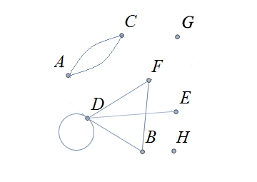
The graph is drawn so that the edge with endpoints \(B\) and \(F\) and the edge with endpoints \(D\) and \(E\) are represented by two line segments that intersect, but the point of intersection is ignored in the graph because it is not a vertex. We could redraw this graph so that the two edges do not cross; for example, we could move \(E\) inside the triangle that has vertices \(B,\) \(D,\) and \(F.\) However, there are some graphs which cannot be drawn in 2 dimensions without some edge crossings.
There is a loop: The edge that has \(D\) as both of its endpoints.
There are parallel edges that connect the vertices \(A\) and \(C,\) so this graph is a multigraph.
Vertex \(G\) is an isolated vertex - it is not an endpoint of any edge. Vertex \(H\) is also an isolated vertex.
This graph is a multigraph because there are multiple edges that connect the pair of vertices \(A\) and \(C.\)
This graph is not a simple graph: It contains a loop, and it has at least one pair of parallel edges.
Notice that in the example and definitions given so far, we’ve assumed that each edge is undirected: An edge represents a connection between its endpoints but does not indicate a direction of travel from one endpoint to the other endpoint. However, in some applications it is useful for a graph to use only directed edges that point from one endpoint to the other endpoint. A graph that has only directed edges is called a digraph, which is short for directed graph.
Most graphs discussed in this chapter will be (undirected) simple graphs, that is, graphs with no loops and no parallel edges.
14.2. The Handshaking Lemma
This section describes a property of every undirected graph.
Recall that the degree of a vertex of a graph is the number of times the vertex occurs as an endpoint for all the edges in the graph. Keep in mind that the vertex of a loop counts twice because that vertex occurs as “both endpoints” of the loop.
Consider again the graph that was drawn in the previous example.
The degrees of each of the vertices in this graph are listed in the table.
| Vertex | Degree |
|---|---|
|
A |
2 |
|
B |
2 |
|
C |
2 |
|
D |
5 |
|
E |
1 |
|
F |
2 |
|
G |
0 |
|
H |
0 |
Notice that the sum of the degrees of all the vertices is \(14\), which is equal to twice the number of edges, \(2 \cdot 7.\)
In fact, for any undirected graph with finitely many edges, the sum of the degrees of all vertices is equal to twice the number of edges (recalling that a loop’s endpoint will be counted twice.)
|
A useful consequence of the Handshaking Lemma is that the sum of the degrees of a graph must be even. |
14.3. Simple Graphs
Recall that in a simple graph, there are no loops and no parallel edges (that is, you cannot have two different edges that connect the same pair of endpoints.) This means that for a simple graph, each edge is determined by its two distinct endpoints. This allows us to give a relatively simple but formal set-theoretic definition of “simple graph.” Graphs discussed in this textbook are assumed to be simple unless stated otherwise.
14.3.1. A Formal Definition of Simple Graph
This subsection presents a formal set-theoretic definition of simple graphs.
A simple graph \(G=\left(V,\ E\right)\) is an ordered pair consisting of a nonempty set \(V\) and a (possibly empty) set \(E,\) where each element of \(E\) must be of the form \(\left\{x,y\right\}\), where \(x\) and \(y\) are two different elements of \(V.\) The elements in set \(V\) are called the vertices (or nodes ) of the graph. The elements in set \(E\) are called the edges of the graph.
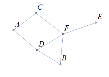
The graph shown has vertex set \(\left\{A,\ B,\ C,\ D,\ E,\ F\right\}\) and edge set \( \{\{A,C\},\{A,D\},\{B,D\},\{B,F\},\{C,F\},\{D,F\},\{E,F\}\}.\)
The degrees of each of the vertices in the undirected graph \(G\) with vertex set \(V=\{A,B,C,D,E,F,G\}\) and edge set \(E=\{\{A,C\},\{A,D\},\{B,D\}\{B,F\},\{C,F\},\{D,F\},\{F,G\}\}\) are,
\(d\left(A\right)=2\)
\(d\left(B\right)=2\)
\(d\left(C\right)=2\)
\(d\left(D\right)=3\)
\(d\left(E\right)=0\)
\(d\left(F\right)=4\)
\(d\left(G\right)=1\)
14.4. Directed Graphs
The main focus of this chapter will be undirected simple graphs, but we will briefly discuss directed graphs in this section.
A directed graph (or digraph ) is a graph in which the edges are directed from one vertex to another vertex. Each edge has an initial vertex \(u\) and a terminal vertex \(v;\) the edge is drawn as an arrow pointing from \(u\) to \(v.\)
The out-degree of a vertex \(w\) is the number of edges that have \(w\) as the initial vertex. The in-degree of a vertex \(w\) is the number of edges that have \(W\) as the terminal vertex.
The directed graph shown has vertex set \(\{A,B,C,D,E,F\}\) and edge set \(\{ (A,C),(D,A),(B,D),(F,B),(C,F),(D,F),(F,E) \}\). The first coordinate of each edge is the initial vertex and the second coordinate is the terminal vertex.
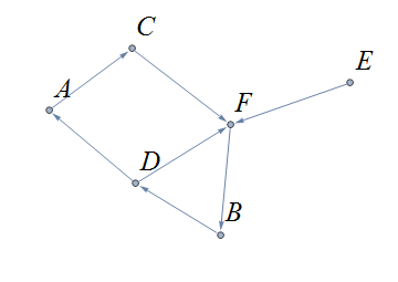
Notice that the directed edges of this graph connect the same endpoints as the undirected edges of the graph in this earlier example. The undirected graph is referred to as the underlying graph of the directed graph.
The graph \(G=(V,E)\) with vertex set \(V = \{ \text{"rock", "paper", "scissors"} \}\) and edge set \(E = \{ \text{("rock", "paper"), ("paper", "scissors"), ("scissors", "rock")} \}\) can be used to represent the game "rock, paper, scissors."
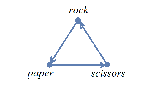
Each directed edge has for its initial vertex the loser and for its terminal edge the winner.
14.4.1. Simple Directed Graphs: A Formal Definition
We can give a formal set-theoretic definition of simple directed graph as well. To indicate the directed edges, ordered pairs of vertices are used instead of 2-element sets.
A simple directed graph \(G=\left(V,\ E\right)\) is an ordered pair consisting of a set \(V\) of objects called vertices (or nodes ) and a set \(E\) of objects called directed edges. Each directed edge \(e\in\ E\) is an ordered pair of the form \(e=\left(x,y\right)\), where \(x\) and \(y\) are two different vertices in set \(V.\) For the directed edge \(e=\left(x,y\right),\) \(x\) is the initial vertex of \(e\) and \(y\) is the terminal vertex of edge \(e\).
14.5. Examples of Simple Graphs
In this section presents several classes of graphs.
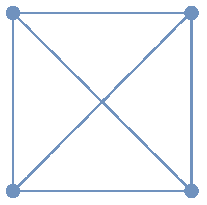
The complete graph \(K_n\) is the simple graph with \(n\) vertices such that any two vertices are adjacent, that is, every pair of vertices are the endpoints of an edge. The image shows \(K_{4},\) the complete graph on 4 vertices. Click here to see images of \(K_{n}\) for the positive integers that are less than or equal to \(12.\)
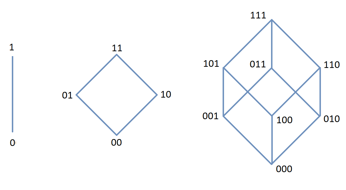
The n-cube \(Q_{n}\) can be described as the graph that has vertex set consisting of the \(2^{n}\) bitstrings of length \(n,\) and edges such that two vertices are adjacent if and only if the bitstrings differ in exactly one bit position. The image shows the three graphs \(Q_{1},\) \(Q_{2},\) and \(Q_{3};\) these graphs can be used as a way to represent the power sets of sets that have \(1,\) \(2,\) and \(3\) elements, respectively. Notice that \(Q_{2}\) can be drawn as a square and that \(Q_{3}\) can be represented as a cube in \(3\)-dimensional space (or by a drawing of a cube in a \(2\)-dimensional plane.)
A bipartite graph is a simple graph whose set of vertices can be partitioned into two disjoint nonempty sets such that every vertex is in exactly one of the two sets and every edge has one endpoint in each of the two sets. One way to think of a bipartite graph is that each vertex can be assigned one of two colors so that every edge must connect vertices of different colors. Notice that \(Q_{1},\) \(Q_{2},\) and \(Q_{3}\) are all examples of bipartite graphs (Question: Is \(Q_{n}\) a bipartite graph for every natural number \(n?\) Why or why not?)
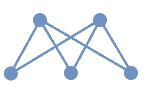
This image shows the graph \(K_{2,3}\) and is another example of a bipartite graph.
Notice that \(K_{2,3}\) has an additional property:
Every
pair of vertices \(\{a, b \}\) with \(a\) in the set of \(2\) "upper" vertices and \(b\) in the set of \(3\) "lower" vertices are the endpoints of an edge. A bipartite graph that has this additional property is called a
complete bipartite graph.
In general, the symbol \(K_{m,n}\) represents the complete bipartite graph that has two disjoint sets of vertices, one of cardinality \(|m|\) and the other of cardinality \(|n|,\) such that every pair of vertices that come from the different sets are joined by an edge. Notice that \(Q_{1} = K_{1,1}\) and \(Q_{2} = K_{2,2}\) are complete bipartite graphs, but that \(Q_{3}\) is not a complete bipartite graph because, for example, there is no edge joining \(000\) and \(111.\)
NOTE: The phrase
"complete bipartite"
needs to be read as a single term used to indicate that a bipartite graph has all the edges it can possibly have. For example, \(K_{2,3}\) is a bipartite graph such that if you tried to enlarge it by inserting an additional edge into the graph, that edge would join either the \(2\) "upper" vertices, \(2\) of the "lower" vertices, or \(2\) vertices that are already joined; in this sense, \(K_{2,3}\) is "complete" as a bipartite graph. \(K_{2,3}\) is not a "complete graph" in the sense of the earlier example in this section. In fact, since a "complete graph" must contain an edge for every pair of distinct vertices, the only graph that can be both a "complete graph" and a "complete bipartite graph" is \(Q_{1} = K_{2} = K_{1,1}.\) Mathematicians recycle and reuse a lot of words… .
14.6. Representing Simple Graphs
In addition to the vertex-edge drawing, a simple graph can be represented in other ways that are more useful for computing.
First, recall that if \(u\) is a vertex of a simple graph, then vertex \(v\) is said to be adjacent to \(u\) if and only if \(\{u, v \}\) are the endpoints of an edge of the graph.
One way to represent a simple graph is by using an adjacency list. This list can be written as a table, where each row has two columns. In each row, the entry in the first column is a single vertex \(v\) and the entry in the second column is a list of all vertices of the graph that are adjacent to \(v.\)
Another way to represent a simple graph is by using an adjacency matrix. The adjacency matrix of a simple graph represents the graph in table form, and contains an entry for each pair of vertices. For each vertex of the graph, there is a row and also a column. If vertices \(u\) and \(v\) are adjacent (that is, connected by some edge), then the adjacency matrix will contain a \(1\) in the position that corresponds to the row for \(u\) and the column for \(v,\) otherwise the matrix contains a \(0\) at that postion. The next example may help make this more clear.
The graph with vertex set \(\left\{A,\ B,\ C,\ D,\ E,\ F\right\}\) and edge set \(\{\{A,C\},\{A,D\},\{B,D\}\{B,F\},\{C,F\},\{D,F\},\{E,F\}\}\) can be represented by
the drawing
or the adjacency list
| Vertex | Adjacent Vertices |
|---|---|
|
A |
C, D |
|
B |
D, F |
|
C |
A, F |
|
D |
A, B, F |
|
E |
F |
|
F |
B, C, D, E |
or the adjacency matrix
\(\mathbf{M}=\left(\begin{matrix}0&0&1&1&0&0\\0&0&0&1&0&1\\1&0&0&0&0&1\\1&1&0&0&0&1\\0&0&0&0&0&1\\0&1&1&1&1&0\\\end{matrix}\right)\)
For example, in matrix \(\mathbf{M}\) the rows, from top to bottom correspond to the vertices \(A,\ B,\ C,\ D,\ E,\ F\) and the columns, from left to right, corespond to vertices \(A,\ B,\ C,\ D,\ E,\ F.\) The values in row 3, which corresponds to vertex \(C\), indicate whether the vertex for that column is adjacent to \(C.\) If we use the symbol \(M_{r,c}\) to stand for the value in row \(r\) and column \(c,\) then \(M_{3,5} = 0\) because there is no edge in the graph with endpoints \(C\) and \(E,\) and \(M_{3,6} = 1\) because there is an edge in the graph with endpoints \(C\) and \(F\).
14.7. Weighted Graphs
In some applications, each edge of a graph has a weight, which is some nonnegative number. The weight could represent the physical distance between the two endpoint nodes, or could represent the cost to travel or transmit data between the endpoint nodes.
You can use an adjacency matrix to describe a weighted graph, but instead of using a \(1\) to represent that there is an edge between two vertices you place the the weight of the edge in the correct position of the adjacency matrix, as shown in the following example.
Consider the following weighted simple graph
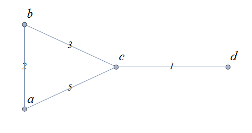
The adjacency matrix of this weighted graph is \( \left(\begin{matrix}0&2&5&0\\2&0&3&0\\5&3&0&1\\0&0&1&0\\\end{matrix}\right). \)
14.8. Creating New Graphs From Old Graphs
Given a set of one or more graphs, there are several ways to create new graphs using the graphs in the set.
14.8.1. Subgraphs
Given a simple graph \(G,\) you can form a
subgraph
\(H\) by choosing a subset of the vertices of \(G\) along with a subset of the edges of \(G\) such that each edge has endpoints in the set of vertices you chose. That is, \(H\) is a subgraph of \(G\) if \(H\) is a graph such that every vertex of \(H\) is a vertex of \(G\) and every edge of \(H\) is an edge of \(G.\)
More formally, \(H = (V_{H}, E_{H})\) is a subgraph of \(G = (V,E)\) if and only if all three of the following statements are True: \(V_{H} \subseteq V,\) \(E_{H} \subseteq E,\) and for every edge \(e \in E_{H}\) the endpoints of \(e\) are in \(V_{H}.\)
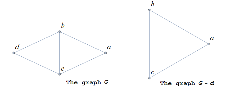
If \(v\) is a vertex of \(G,\) we denote by \(G-v\) , the subgraph obtained from \(G\) by removing the vertex \(v\) along with all edges in \(E\) that have \(v\) as an endpoint.
The image shows a graph \(G\), and the subgraph \(G-d\) formed by removing the vertex \(d\).
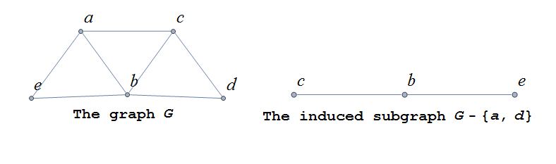
In the same way, you can obtain a subgraph by removing multiple vertices along with the edges associated with the removed vertices. The subgraph obtained is called the subgraph induced by removing those vertices.
Below is a graph \(G(V,E)\) and the subgraph obtained by \(V-\{a,d\}\), called the induced subgraph \(G-\{a,d\}\), with a slight abuse of notation
14.8.2. Unions and Intersections Of Graphs
Given two simple graphs \(G_{1}\) and \(G_{2}\), you can form the union of the graphs by taking the union of the two sets of vertices to get a new set of vertices, and taking the union of the two sets of edges to get a new set of edges. Notice that any edge that is in both graphs will only appear once in the new graph because you took the union of the sets of edges, that is, you can’t create parallel edges by forming the union.
In the same way, you can form the intersection of two simple graphs by taking the intersection of the two sets of vertices to get a new set of vertices, and taking the intersection of the two sets of edges to get a new set of edges.
14.9. Graph Isomorphism
Recall that a graph is determined by its set of vertices and how those vertices are connected by edges, but not the drawing you use to represent the graph.
Consider the two graphs shown in the image.
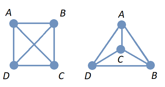
Notice that these two graphs are different-looking drawings of the same graph that has vertex set \(\{ A, B, C, D\}\) and edge set \(\{\{A,B\},\{A,C\},\{A,D\},\{B,C\},\{B,D\},\{C,D\}\}.\) Also, notice that the drawing on the left appeared earlier in the chapter, but with unlabeled vertices: Each of the graphs in the image is a drawing of \(K_{4},\) the complete graph on \(4\) vertices.
Notice that using either the adjacency list
| Vertex | Adjacent Vertices |
|---|---|
|
A |
B, C, D |
|
B |
A, C, D |
|
C |
A, B, D |
|
D |
A, B, C |
or the adajcency matrix \[\left(\begin{matrix}0&1&1&1\\1&0&1&1\\1&1&0&1\\1&1&1&0\\\end{matrix}\right)\] makes it easier to see that the two drawings represent the exact same graph.
You can imagine the graph on the right being the result of dragging the vertex \(C\) inside the "triangle" with vertices \(A,\) \(B,\) and \(D.\)
Sometimes, different graphs may be essentially the same graph, as in the next example.
Consider the two graphs, each with \(4\) vertices and \(6\) edges, shown in the image.
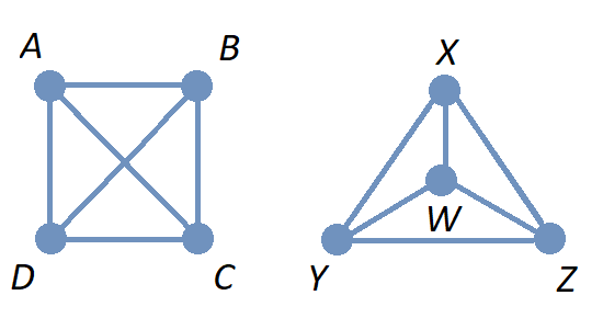
These graphs are not equal since the graph on the left has vertex set \(\{ A, B, C, D\}\) and the graph on the right has vertex set \(\{ W, X, Y, Z\}.\) However, by comparing the graph on the right to the one on the right in the previous example, you can see that there is a one-to-one correspondence between the two sets of vertices that preserves adjacency (that is, if two vertices in the upper row are endpoints of an edge of the graph on the left, then the corresponding vertices in the lower row are endpoints of an edge of the graph on the right.)
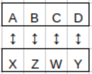
A one-to-one correspondence between the set of vertices of two simple graphs that preserves adjacency is called a graph isomorphism, and the two graphs are said to be isomorphic. That is, two vertices are endpoints of an edge in the first graph if and only if the corresponding vertices are the endpoints of an edge in the second graph. Informally, you can think of two isomorphic graphs as a pair of graphs where a drawing of one graph can be relabeled and/or reshaped to obtain a drawing of the other graph (That is, the two graphs are really the same graph but have drawings that are labeled and/or shaped differently.)
Using graph isomorphisms can help identify properties of a graph.
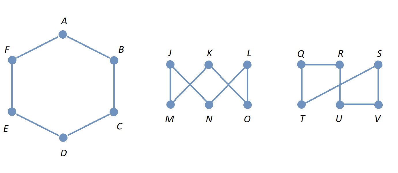
The three graphs in the image are isomorphic; it is an exercise for you to write out the one-to-one correspondences.
Write out the one-to-one correspondences between the sets of vertices that define the graph isomorphisms.
Once you have shown that the three graphs are isomorphic, you can use the fact that they are different representations of the same graph. For example,
-
It is not immediately clear that the graphs on the left and right are bipartite, but the arrangement of the vertices in the middle graph into "upper" and "lower" rows makes this easy to see.
-
Also, it is not immediately clear that the graph in the middle or the graph on the right is planar (that is, the graph can be redrawn in a \(2\)-dimension plane so that no edges cross) but this is obvious for the graph on the left.
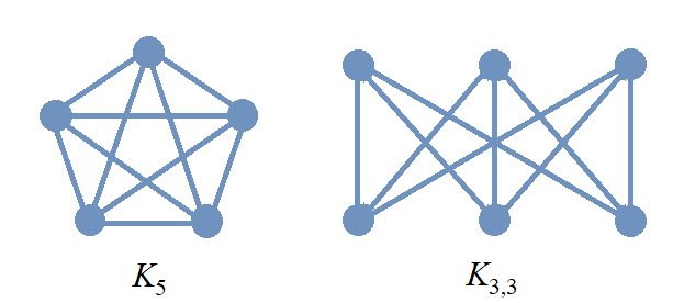
This textbook does not discuss planar graphs in detail, but it is worth mentioning that it can be proven that neither \(K_{5}\) nor \(K_{3,3}\) is planar. If you’d like to learn more about planar graphs, one source is the section "Planar Graphs" in Oscar Levin’s Discrete Mathematics: An Open Introduction, 4th edition. |
14.9.1. Isomorphism of Graphs with Additional Features
As described above, a graph isomorphism is a one-to-one correspondence between the sets of vertices of two graphs that preserves the adjacency relationship between pairs of vertices. That is, two vertices are endpoints of an edge in one graph if and only if the corresponding vertices are endpoints of an edge in the other graph.
In cases where graphs have additional features beyond the basic adjacency relationship between pairs of vertices, we should only consider two of these “graphs with additional features” to be isomorphic if the additional features are also preserved.
Note: Some sources use the word “attributes” for these additional features.
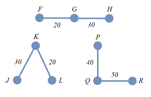
As an example, in the image, the three graphs with vertex sets \(\{ F,\,G,\,H \},\) \(\{ J,\,K,\,L \},\) and \(\{ P,\,Q,\,R \}\) are isomorphic as graphs if we ignore the edge weights. Also, the two graphs with vertex sets \(\{ F,\,G,\,H \}\) and \(\{ J,\,K,\,L \}\) are isomorphic as weighted graphs because there is a one-to-one correspondence between the vertex sets that preserves both the adjacency relationships and the corresponding edge weights. The third graph with vertex set \(\{ P,\,Q,\,R \}\) is not isomorphic as a weighted graph to either of the other two weighted graphs because its edge weights cannot be matched with the edge weights in the other weighted graphs.
14.10. Graph Coloring
In some contexts, it can be useful to partition either the set of vertices or the set of edges of a graph into disjoint subsets to make it easier to understand the graph and the network it represents. This act of partitioning is usually referred to as "coloring" since using different colors can make it easy to see and interpret the properties of the partition when the graph is drawn. Notice that you could instead create the partition by assigning labels like "group 1," "group 2," and so on, to each vertex (or edge.)
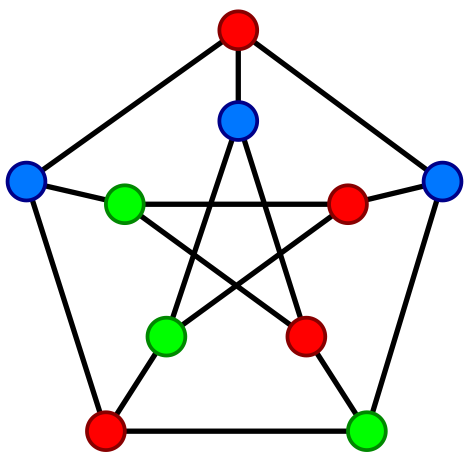
For example, the image shows a graph called the Petersen graph with its vertex set partitioned into 3 subsets so that each edge’s endpoints are in two different subsets of the partition (That is, each edge’s endpoints have different colors.)
Image credit:
"Petersen_graph_3-coloring.svg"
by Д.Ильин. The copyright holder of this work has released this work into the public domain. This applies worldwide.
The next example discusses an application of vertex coloring.
The following image represents a "map" showing four countries; the blue region represents one country (not a body of water) that is surrounded by three other countries.
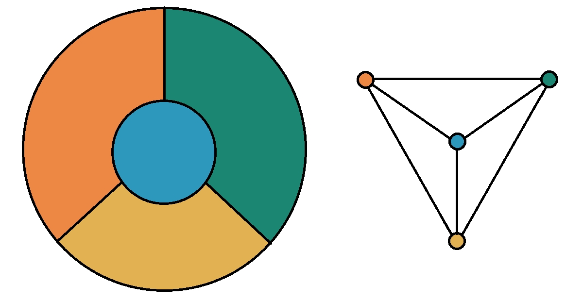
The map can be represented as a graph with vertices colored to match the regions, as shown on the right. If it helps you to connect the graph to the map, imagine that each vertex represents a capital city of the corresponding country.
This way of representing a map was used to prove the Four Color Theorem which states, roughly, that
Any map of countries that can be drawn in a plane such that
(1) every country has a color and
(2) no two adjacent countries have the same color
requires at most four different colors.
In this context "two adjacent countries" share a border that is not just a single point.
The first proof of the theorem was announced in 1976, and a corrected version of the first proof was published in 1989 after some errors were fixed (Yes, professional mathematicians do make mistakes!) The proof was considered controversial by many mathematicians at the time because it was the first major computer-assisted proof: Over one thousand five hundred different cases needed to be checked!
In other contexts, it is more appropriate to use edge coloring. That is, each edge of the graph is assigned a color so that the set of edges is partitioned into disjoint subsets.
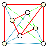
For example, the graph in the image shows that the complete bipartite graph \(K_{4,4}\) can be partitioned as a union of 3 disjoint graphs called
forests
(Forests are defined later in this textbook, in the
Trees
chapter.)
Image credit:
"K44 arboricity.svg"
by David Eppstein. The copyright holder of this work has released this work into the public domain. This applies worldwide.
14.11. Connectivity of Undirected Graphs
A walk on a graph \(G=\left(V,E\right)\) is a finite, non-empty, alternating sequence of vertices and edges of the form, \(v_0e_1v_1e_2\ldots e_nv_n\), with vertices \(v_i\in V\) and edges \(e_i\in E\), where for each integer value of \(i \leq n\) the endpoints of \(e_i\) are the vertices \(v_{i-1}\) and \(v_i.\) The integer \(n\) is called the length of the walk.
If we restrict ourselves to simple undirected graphs, there is at most one edge joining each pair of adjacent vertices, so a walk can be specified simply by listing the sequence of vertices \(v_0v_1\ldots v_n\) (That is, we don’t need to write down the edges.)
-
A trail is a walk that does not repeat an edge. That is, all edges in a trail are distinct.
-
A path is a trail that does not repeat a vertex (but we allow for the possibility that the initial vertex \(v_0\) and terminal vertex \(v_n\) of the path are the same vertex; When \(v_0=v_n\) the path is called a closed path or a circuit. )
-
A cycle is a closed path of length at least 1.
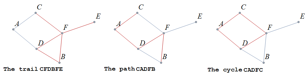
The distance \(d(u,v)\) between two vertices \(u\) and \(v\) in a graph \(G\) is the number of edges in a shortest path connecting them, assuming such a path exists.
In the graphs below the first shows a trail \(CFDBFE\). It is not a path since the vertex \(F\) is repeated. The second shows a path \(CADFB\), and the third a cycle \(CADFC\). Also note the following distances, \(d(A,D)=1\), while \(d(A,F)=2\), and \(d(A,E)=3\).
14.12. Connected Graphs
A graph \(G\) is connected if there is a path between any pair of vertices.
The graph \(G\) below is not connected since, as just one example, there is no path between vertex \(a\) and vertex \(e.\)
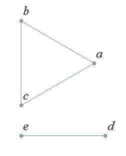
\(G\) has adjacency matrix
\( \left(\begin{matrix}0&1&1&0&0\\1&0&1&0&0\\1&1&0&0&0\\0&0&0&0&1\\0&0&0&1&0\\\end{matrix}\right). \)
In the previous example, the graph \(G\) can be treated as a union of two connected subgraphs, called the connected components of \(G.\) It can be proven by mathematical induction that any simple undirected graph that has a finite number of vertices can be written as a union of a finite number of connected components.
14.13. Eulerian Graphs
An Euler path on a graph is a path that uses each edge of the graph exactly once.
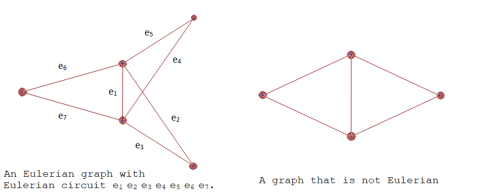
An Euler circuit (also called an Eulerian trail ) is a closed trail containing each edge of the graph \(G\) exactly once and returning to the start vertex. A graph with an Euler circuit is called Eulerian or is said to be an Eulerian graph .
In the following, the first graph is Eulerian. The sequence of edges \(e_1 e_2 e_3 e_4 e_5 e_6 e_7\) describes an Euler circuit (Notice that some vertices are visited multiple times; it is the edges that must appear exactly once in an Euler path.) The second graph is not an Eulerian graph. Convince yourself of this fact by looking at all necessary trails or closed trails.
The following are useful characterizations of graphs with Euler circuits and Euler paths and are due to Leonhard Euler
Euler solved a famous problem about the seven bridges of Königsberg by representing the problem as a graph (with parallel edges.)
14.14. Hamiltonian Graphs
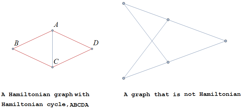
A cycle in a graph \(G\), is called a Hamiltonian cycle if every vertex, except for the starting and ending vertex, is visited exactly once.
A graph is Hamiltonian , or said to be a Hamiltonian graph , if it contains a Hamiltonian cycle.
The following graph is Hamiltonian and shows a Hamiltonian cycle \(ABCDA\), highlighted (Notice that some edges are used multiple times; it is the vertices, starting and ending vertex, that must appear exactly once in an Hamiltonian path.) The second graph is not Hamiltonian.
14.15. Finding A Shortest Path in a Weighted Graph: Dijkstra’s Algorithm
In some applications of graph theory, you need to find a "shortest path" between two vertices of a weighted graph. In the context, shortest may mean "of least distance" but could mean "of least cost" or something else, depending on what the edge weights represent.
Edsger Dijkstra published a
paper
in 1959 that describes an algorithm for finding the path of "minimum total weight" between two given vertices of a simple connected graph with weighted undirected edges.
Dijkstra’s original paper is also available in the ACM Digital Library at
this link.
Here is a description of the algorithm, based on Dijkstra’s original.
-
Task: Given two vertices \(a\) and \(z,\) find the edges of a path between the two vertices that has the minimum possible sum of weights.
-
Input: The list \(V\) of all vertices of the graph, with the two vertices \(a\) and \(z\) specified, and the list \(E\) of all weighted edges of the graph.
For example, the input could be an adjacency matrix for the graph, with the first row of the matrix corresponding to \(a\) and the last row corresponding to \(z\). -
Steps:
-
Define four lists \(V_{chosen},\) \(V_{candidates},\) \(E_{chosen},\) and \(E_{candidates},\) and initialize each list as an empty list.
-
Append vertex \(a\) to the end of \(V_{chosen}.\)
-
While vertex \(z\) has not been appended to \(V_{chosen}\)
-
Set \(v\) to the last vertex appended to \(V_{chosen}.\)
-
For each vertex \(w\) that is not in \(V_{chosen}\) but is adjacent to vertex \(v\)
-
If \(w\) is in \(V_{candidates}\) and the edge \(e\) that connects \(v\) and \(w\) is part of a path between \(a\) and \(w\) that has total weight less than the weight of the known path that uses the corresponding edge in list \(E_{candidates},\) remove that edge from \(E_{candidates}\) and append \(e\) to \(E_{candidates}.\)
-
Otherwise, \(w\) is in neither list \(V_{chosen}\) nor list \(V_{candidates},\) so append vertex \(w\) to the end of \(V_{candidates}\) and append the edge \(e\) that connects \(v\) and \(w\) to the end of \(E_{candidates}.\)
-
-
After exiting the "for" loop,
-
find the vertex \(w\) in list \(V_{candidates}\) that has the minimal-weight path to the starting vertex \(a\) and append \(w\) to the end of \(V_{chosen},\) and remove \(w\) from \(V_{candidates},\) and
-
append the edge in \(E_{candidates}\) that has \(w\) as one of its endpoints to the end of \(E_{chosen}\) and remove that edge from \(E_{candidates}.\)
-
-
-
-
Output: The list \(E_{chosen}\) of weighted edges.
Notice that the list \(E_{chosen}\) is constructed so that it contains edges for only one possible path between \(a\) and \(z,\) and that path must be a minimal-weight path.
Also notice if the loop condition is changed to "while there is a vertex that is not in \(V_{chosen}\)" then the algorithm’s output \(E_{chosen}\) will find the edges needed for a possible minimal-weight path between vertex \(a\) and any other vertex in the graph.
Question: What change would be needed to the input if you had a graph with unweighted edges and needed to find a path between \(a\) to \(z\) that uses the smallest number of edges possible?
This Wikipedia page has some animations that illustrate an alternate implementation of Dijkstra’s algorithm.
14.16. The Traveling Salesperson Problem (TSP)
The Traveling Salesperson Problem (TSP) can be stated as “A traveling salesperson needs to start in the home city, visit each of a number of other cities, and then return to the home city. What path should the salesperson take so that the total distance traveled is the least possible?”
The TSP can be modeled using a graph. If there are \(n\) cities, you can represent each city as a vertex of the complete graph \(K_{n}\) and assign to each edge a weight equal to the distance between the cities at the endpoints. The TSP is solved by finding a Hamiltonian cycle of minimum total weight that visits each vertex exactly one.
Notice that if you choose a vertex (city) as the starting and ending point, then there are \(\frac{1}{2}(n-1)!\) different Hamiltonian cycles (The division by 2 represents that you could reverse the direction of the cycle without changing the total distance traveled.)
The brute-force solution examines every possible path and has time complexity \(\Theta (n!),\) which is infeasible for even relatively small values of \(n.\) There is the Bellman–Held–Karp algorithm that solves the TSP with time complexity \(\Theta (2^{n}n^{2}).\) Also, there are other methods to find “approximate” solutions to the TSP that are “good enough” for some problems. At present, there is no known algorithm with polynomial worst-case time complexity that solves the TSP.
14.17. Additional topics will be added to this chapter soon!
-
Transitive closure (Floyd’s algorithm)
-
Topological sort
MORE TO COME!