Discrete Math - The MKD Remix (CSC230 Version)

15. Trees

CAUTION - CHAPTER UNDER CONSTRUCTION!

NOTICE: If you are NOT enrolled in the CSC 230 course that I teach at SFSU, you probably are looking for the “public version” of the book, which I only update between semesters. The version you are looking at now is the “CSC230 version” of the book, which I will be updating throughout the semester.

This chapter was last updated on December 8, 2025.
Added more content to the section on binary trees: Tree traversal algorithms, Łukasiewicz’s parentheses-free notation (“Polish notation”) and expression trees.
Revised section on directed trees. Rewrote theorem on second characterization of trees.

A tree is a connected simple graph that contains no cycles. Trees are used to model decisions, to sort data, and to optimize networks.

Key terms and concepts covered in this chapter:

Trees
- Definition of “tree” and “forest”
- Properties of trees
- Spanning trees
- Binary trees
  - Traversal strategies
  - Expression trees

15.1. Definitions, Examples, and Properties of Trees and Forests

In this section, you will learn some of the basics about trees.

Much of the terminology related to trees is not standardized, that is, different textbooks and sources use different terminology for the same types of trees. The Remix uses terminology consistent with Handbook of Graph Theory, Second Edition by Gross, Yellin, and Zhang.

Recall that a simple graph has no loops and no parallel edges.

Also, recall that a cycle in a graph is a path that starts and ends at the same vertex.

A tree is a simple graph that is connected and has no cycles. Some sources use the term acyclic to mean "has no cycles."

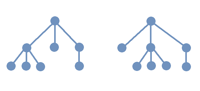
A forest is the union of several trees. In other words, a forest is a simple graph that has one or more connected components, where each connected component is a tree.

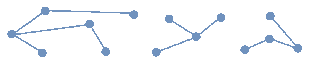
The image shows a forest composed of three trees.

Notice that if you choose any pair of vertices in one of the trees in the image, there is only one path that joins that pair of vertices. In fact, this property is True for any tree.

Theorem

Suppose that \(G\) is a simple graph. The following statements are logically equivalent.

\(G\) is a tree.
\(G\) is a simple graph such that for each pair of vertices of \(G\) there is exactly one path between the vertices.

Proof

First, assume that \(G\) is a tree; we will prove, using proof by contradiction, that for every pair of vertices of \(G\) there is exactly one path between the vertices. By assumption, \(G\) is connected and for every pair of vertices in \(G\) there is at least one path joining those two vertices, so we only need to show that there cannot be two different paths that connect the same pair of vertices. To work toward a contradiction, let’s suppose that for some pair of vertices \(u\) and \(v\) there are two different paths between \(u\) and \(v;\) then we can start to go from \(u\) to \(v\) along a first path and then “turn around and go back” to \(u\) along a second path. This means that there must be a cycle in \(G\) that starts and ends at \(u.\)

Why must there be a cycle?

If we can go all the way from \(u\) to \(v\) along the first path and then go all the way back, in reverse order, from \(v\) to \(u\) along the second path without repeating any edges or vertices (except \(u\)) then we have found a cycle that starts and ends at \(u.\)
If the two paths have some common edges or vertices, we can use only part of each path to create a cycle that does not repeat any edges or vertices. To do this, write the first path as \(v_{0}v_{1}...v_{n-1}v_{n}\) where \(u = v_{0}\) and \(v = v_{n}\) and let \(j\) stand for the smallest positive index such that vertex \(v_{j}\) appears in both the first and second paths. Now create a cycle by using the beginning of the first path to go from \(u\) to \(v_{j}\) and then using the beginning part of the second path that goes from \(u\) to \(v_j\), but in reverse order, to go back from \(v_{j}\) to \(u.\) Notice that the index \(j\) is chosen so that that no edge or vertex (except \(u\) and \(v_j\)) that we use can belong to both of these shorter paths from \(u\) to \(v_{j},\) so no edges are repeated when we use this path to go from \(u\) back to \(u\) - we have created a cycle.

To continue with the proof by contradiction, we’ve shown that there is a cycle in \(G,\) but this contradicts the assumption that \(G\) is a tree that has no cycles. This means that the assumption "there is a pair of vertices in \(G\) that are connected by two different paths" must be False. We have proven that for any pair of vertices in \(G\) there is exactly one path joining that pair of vertices.

Secondly, assume that \(G\) is a simple graph and that for every pair of vertices of \(G\) there is exactly one path between the vertices. We will prove, using proof by contradiction, that \(G\) must be a tree. By assumption, \(G\) is connected because for any pair of vertices there is a path between those vertices, so we only need to prove that \(G\) has no cycles. To reach a contradiction, let’s suppose that \(G\) does have a cycle of the form \(v_{0}v_{1} \cdots v_{n-1}v_{n}\) where \(v_{0} = v_{n}\) (that is, \(v_{0}\) and \(v_{n}\) are the same vertex, but no other vertex is repeated in the cycle.) Notice that, because \(G\) is a simple graph, the integer \(n\) must be greater than or equal to 3.

Why must n be greater than or equal to 3?

Notice that \(n\) must be positive since there are at least two vertices in the path.
If \(n=1\) then the cycle is \(v_{0}v_{1}\) where \(v_{0} = v_{1},\) but this cycle consists of a single loop, which contradicts that \(G\) is a simple graph that has no loops.
If \(n=2\) then the cycle is \(v_{0}v_{1}v_{2}\) where \(v_{0} = v_{2},\) but this cycle would use the same edge twice which contradicts the definition of a cycle.
This shows that \(n \geq 3.\)

This means that we have two different paths, \(v_{0}v_{1}\) and \(v_{1} \cdots v_{n},\) between \(v_0\) and \(v_1\) (because \(v_{0}\) and \(v_{n}\) are the same vertex.) Now we can reverse the order of vertices in the second path to get two different paths between the vertices \(v_{0}\) and \(v_{1}\) - but we assumed that for every pair of vertices of \(G\) there is exactly one path between those vertices. We have derived a contradiction, which means that \(G\) cannot have a cycle. Therefore, \(G\) is connected and has no cycles, which is the definition of a tree, so \(G\) is a tree.

Q.E.D.

Next, we will give another characterization of trees, after first proving a lemma.

Lemma

Suppose that \(G\) is a connected simple graph with \(n\) vertices and \(n-1\) edges, where \(n\) is some postive integer greater than or equal to \(2.\) Then \(G\) must have at least one vertex of degree \(1.\)

Proof

\(G\) is assumed to be a connected graph, so that every vertex is the endpoint of at least one edge. That is, the degree of every vertex is greater than or equal to \(1.\)

We now use proof by contradiction to show that there is at least one vertex that has degree equal to \(1.\) To work towards a contradiction, suppose that every vertex has degree greater than \(1,\) that is, the degree of every vertex is greater than or equal to \(2.\) This means that the sum of the degrees of all vertices is greater than or equal to \(2n.\) By the Handshake Lemma, the sum of the degrees of the vertices must be equal to \(2\) times the number of edges, which in this case is \(2(n-1).\) We have obtained a contradiction, since the Handshake Lemma proves that the sum of the degrees of the vertices must be equal to \(2(n-1)\), but the sum of the degrees of the vertices must also be greater than or equal to \(2n.\) From this contradiction we can conclude that it is False that the degree of every vertex is greater than or equal to \(2,\) so there must be at least one vertex with degree less that \(2.\) Recalling that the degree of every vertex is greater than or equal to \(1\) proves that at least one vertex has degree \(1.\)

Theorem

Suppose that \(G\) is a connected simple graph with finitely many vertices. The following statements are logically equivalent.

\(G\) is a tree.
If \(G\) has \(n\) vertices, where \(n\) is a positive integer, then \(G\) has \(n-1\) edges.

Proof

First, assume \(G\) is a tree with \(n\) vertices. We will use mathematical induction on \(n\) to prove that the number of edges must be \(n-1.\)

Let \(P(n)\) be the predicate \[P(n): \text{If a tree has } n \text{ vertices then the tree has } n-1 \text{ edges.}\] We will prove that the proposition \((\forall n \in \mathbb{N}_{>0})P(n)\) is True.

Basis Step: \(P(1)\) is True since a tree that has \(1\) vertex has \(0\) edges (otherwise, the edge would have to be a loop, but trees are simple graphs that don’t have loops.)
We can also prove that \(P(2)\) is True in case the proof of \(P(1)\) feels unsatisfying. If a tree has \(2\) vertices, then since a tree is a connected simple graph, the \(2\) vertices must be connected by a path, and since a tree cannot have parallel edges, the vertices are the endpoints of exactly \(1\) edge. This proves that \(P(2)\) is True.

Induction Step: First, we assume that the induction hypothesis \(P(k)\) is True for some positive natural number \(k\).

Secondly, we will prove that the conditional \(P(k) \rightarrow P(k+1)\) must be True, which means we can use modus ponens (or the equivalent tautology \(( P(k) \land ( P(k) \rightarrow P(k+1) ) ) \rightarrow P(k+1)\)) to show that \(P(k+1)\) is also True.

Assume that \(P(k)\) is True for the positive integer \(k,\) that is, if a tree has \(k\) vertices then the tree has \(k-1\) edges. We can assume \(k \geq 2\) since the cases when \(k \in \{ 1, 2 \}\) were proved in the Basis Step. Suppose that we have a tree \(T\) that has \(k+1\) vertices; we will prove that the tree must have \(k\) edges. First, there must be at least one vertex \(v\) in \(T\) such that the degree of \(v\) is 1: If every vertex had at least degree \(2,\) then we could find a cycle in \(T,\) which cannot be True since \(T\) is a tree. Remove one vertex \(v\) that has degree \(1\) along with the edge that has \(v\) as an endpoint to obtain the subgraph \(T-v.\) Notice that for every pair of vertices of \(T-v\) there is exactly one path between the vertices, and applying the previous theorem shows that \(T-v\) is a tree. Also, \(T-v\) has \(k\) vertices because we removed only \(v,\) so we can apply the Induction Hypothesis to conclude that \(T-v\) has \(k-1\) edges. Now, reinsert vertex \(v\) and the edge that was removed to obtain the tree \(T\) that has \(k+1\) vertices and \(k\) edges. Therefore, if \(P(k)\) is True then \(P(k+1)\) is True, too. That is, \(P(k) \rightarrow P(k+1)\).

Conclusion Step: We have proven both the Basis Step and the Induction Step. Therefore, we can conclude that for all positive integers \(n,\) if a tree has \(n\) vertices then the tree has \(n-1\) edges.

Secondly, assume that \(G\) is a connected simple graph that has a finite number of vertices such that the number of edges is one less than the number of vertices. We will use mathematical induction on the number of vertices to prove that \(G\) is a tree.

Let \(P(n)\) be the predicate \[P(n): \text{If } G \text{ is a connected simple graph that has } n \text{ vertices and } n-1 \text{ edges then } G \text{ is a tree.}\] We will prove that the proposition \((\forall n \in \mathbb{N}_{>0})P(n)\) is True.

Basis Step: \(P(1)\) is True since a connected simple graph that has \(1\) vertex and \(0\) edges is a tree.
We can also prove that \(P(2)\) is True in case the proof of \(P(1)\) feels unsatisfying. If G is a connected simple graph that has \(2\) vertices and \(1\) edge, then the edge cannot be a loop so must have \(2\) different endpoints. Since there are only \(2\) vertices in \(G\), the edge must have those vertices as its endpoints, so \(G\) consists of a single edge with distinct endpoints. Since there is exactly one path from one of the vertices to the other, the previous theorem can be applied to show that \(G\) is a tree. This proves that \(P(2)\) is True.

Induction Step: First, we assume that the induction hypothesis \(P(k)\) is True for some positive natural number \(k\).

Assume that \(P(k)\) is True for the positive integer \(k,\) that is, if a connected simple graph has \(k\) vertices and \(k-1\) edges then the graph is a tree. We can assume \(k \geq 2\) since the cases when \(k \in \{ 1, 2 \}\) were proved in the Basis Step. Suppose that we have a connected simple graph \(G\) that has \(k+1\) vertices and \((k+1)-1\) edges; we will prove that \(G\) is a tree. From the lemma proved earlier, we know that at least one of the vertices in \(G\) must have degree exactly equal to \(1;\) let \(v\) be such a vertex. Now consider the graph \(G-v\) obtained by removing \(v\) and the one edge \(e_v\) that has \(v\) as an endpoint: It is a connected simple graph with \(k\) vertices and \(k-1\) edges, so the Induction Hypothesis lets us conclude that \(G-v\) is a tree. In particular, there is exactly one path between any two vertices in \(G-v.\) Now reattach \(v\) and the edge \(e_v\) that has \(v\) as an endpoint. Notice that there is exactly one path between any two vertices in \(G:\) Either the two vertices are in \(G-v\) (so there is exactly one path) or one vertex, \(w,\) is in \(G-v\) and the other vertex is \(v,\) but in this second case there is exactly one path which goes from \(v\) to the other endpoint of the edge \(e_v\) and then continues as a path in \(G-v\) from that other endpoint to the vertex \(w.\) Since there is only one path between \(w\) and the other endpoint of \(e_v\) in \(G-v,\) this path between \(w\) and \(v\) is the only one possible path in \(G.\) In summary, we have shown that there is exactly one path between any two vertices in \(G,\) and the previous theorem applies to prove that \(G\) is a tree.

Q.E.D.

15.2. Spanning Trees and Spanning Forests

Recall that a subgraph of a graph \(G\) is a graph \(H\) such that every vertex of \(H\) is a vertex of \(G\) and every edge of \(H\) is a edge of \(G\) (with both endpoints in the vertex set of \(H.\))

A subtree of a graph \(G\) is a subgraph of \(G\) that is also a tree. Likewise, a subforest of \(G\) is a subgraph of \(G\) that is also a forest.

A spanning tree of a graph \(G\) is a subgraph of \(G\) that is a tree that includes all the vertices of \(G.\) Likewise, a spanning forest of a graph \(G\) is a subgraph of \(G\) that is a forest that includes all the vertices of \(G.\)

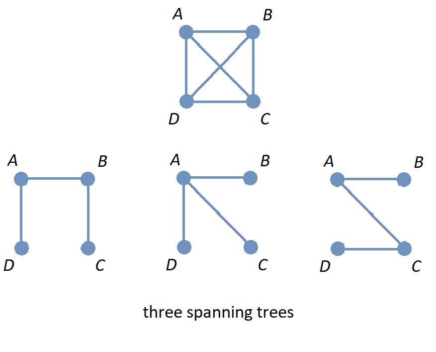
The image shows the graph \(K_{4}\) along with three spanning trees.

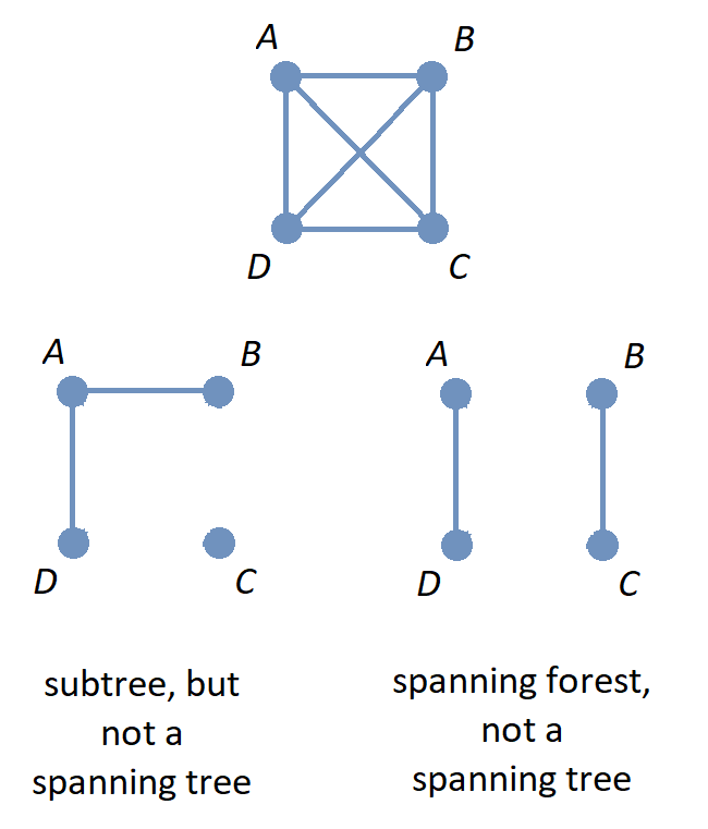
The image shows the graph \(K_{4}\) along with a subgraph that is a subtree that is not a spanning tree, and also a subgraph that is a spanning forest.

Spanning trees are used to solve problems that involve simplifying or optimizing networks. You can learn more about some of the applications of spanning trees at this Wikipedia page.

The following subsection presents one such application.

15.2.1. Minimal-Weight Spanning Trees in Weighted Graphs

In some applications of graphs with weighted edges, you may need to find a spanning tree that has the minimal total weight possible, that is, a spanning tree with sum of edge weights less than or equal to the corresponding sum for any other spanning tree. Such a spanning tree is referred to as a minimal-weight spanning tree.
Note: Many textbooks and sources use the term minimum length spanning tree because the use of these spanning trees historically arose in problems that involved physical distances between nodes of a network. Other sources use the term minimum spanning tree, abbreviated as MST.

As an example, the image shows a weighted graph along with all three possible spanning trees. The minimal-weight spanning tree, with total weight 6, is drawn on the lower left.

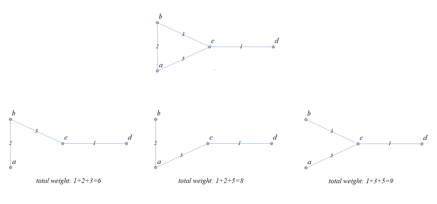
Notice that for the graph in the image, it was both easy and efficient to use “brute force” to look at all of the spanning trees and compute all of the sums of weights for those spanning trees. For weighted graphs that have many more vertices and/or edges, you will need to use a more efficient problem-solving strategy. This textbook discusses one such strategy, Kruskal’s algorithm, in detail.

Kruskal’s Algorithm

Joseph Kruskal published a paper in 1956 that describes an algorithm for constructing “the shortest spanning subtree” of a connected simple graph (Kruskal assumed that the graph has only finitely-many edges, and that each edge has a positive weight which represents the distance between its endpoints.)

Task: Given a connected graph \(G = (V,E)\) with weighted edges, construct a spanning tree of \(G\) that has the minimal possible sum of weights.
Input: The list \(E\) of all weighted edges of the graph.
Steps:
1. Sort the list of edges \(E\) so that each edge \(e_{k}\) in the list has a weight that is less than or equal to the next edge \(e_{k+1}\) in the list.
2. Define the list \(E_{chosen}\) and initialize it as an empty list.
3. Set integer index variable \(i\) to 0.
4. While \(i\) is less than \(|E|,\) the number of edges
  1. If it is impossible to form a cycle using edge \(e_{i}\) along with some (or all) of the edges in list \(E_{chosen}\)
    
    Append \(e_{i}\) to \(E_{chosen}\)
  2. Increment \(i\) by 1
Output: The list \(E_{chosen}\) of weighted edges.

Notice that the output list \(E_{chosen}\) was constructed so that its edges cannot be used to form a cycle in the graph \(G.\) Also, since the graph \(G\) is assumed to be connected, every vertex will be the endpoint of at least one edge in \(E_{chosen},\) so that the graph with vertex set \(V\) and edge set \(E_{chosen}\) will be a spanning tree of \(G.\)

Also notice that the condition for the while loop can be changed to “while \(|E_{chosen}| < |V| - 1\)” since a spanning tree must have one fewer edges than vertices.

Example 1 - An example of using Kruskal’s algorithm

The image shows a drawing of a simple weighted graph along with all three possible spanning trees.

The minimal-weight spanning tree, with total weight 6, is drawn on the lower left.

Let’s trace through the steps of Kruskal’s algorithm to examine how this minimal-weight spanning tree is constructed. The following table represents the input to the algorithm: A list of all the edges of the graph, along with their corresponding weights.

Edge	Weight
{c, d}	1
{a, b}	2
{b, c}	3
{a, c}	5

Steps:
1. Sort the list of edges of the graph in order of increasing weight (This has already been done in the table shown.)
2. Set \(E_{chosen}\) to the empty list.
3. Set the index \(i\) to 0.
4. Enter the while loop.
  
  \(i=0\)
  
  \(i\) is less than 4, and it is impossible to form a cycle using \(\{c, d\}\) alone,
  so set \(E_{chosen}\) to \([\{c, d\}\)] and set \(i\) to 1.
  
  \(i=1\)
  
  \(i\) is less than 4, and it is impossible to form a cycle using \(\{a, b\}\) along with the edge in \(E_{chosen} = [\{c, d\}\)]
  so set \(E_{chosen}\) to \([\{c, d\} , \{a, b\}\)] and set \(i\) to 2.
  
  \(i=2\)
  
  \(i\) is less than 4, and it is impossible to form a cycle using \(\{b, c\}\) along with the edges in \(E_{chosen} = [\{c, d\} , \{a, b\}\)]
  so set \(E_{chosen}\) to \([\{c, d\} , \{a, b\}, \{b, c\}\)] and set \(i\) to 3.
  
  \(i=3\)
  
  \(i\) is less than 4, but it is possible to form a cycle using \(\{a, c\}\) along with the edges in \(E_{chosen} = [\{c, d\} , \{a, b\}, \{b, c\}\)]
  so make no change to \(E_{chosen}\) and set \(i\) to 4.
  
  \(i=4\)
  
  Since \(i\) is not less than 4, exit the while loop.

The output is \(E_{chosen} = [\{c, d\} , \{a, b\}, \{b, c\}\)] which is the list of edges used in the spanning tree drawn on the lower left of the image. That is, in at least this one case, the algorithm does construct a minimal-weight spanning tree.

Question

How could you validate Kruskal’s algorithm?
That is, how could you prove that Kruskal’s algorithm must construct a minimal-weight spanning tree for any input graph that is connected and has finitely-many weighted edges?

Hint

Try to create a predicate that you could prove True for all natural numbers by using mathematical induction.

Here is an exercise for you to try.

Check Your Understanding

Use Kruskal’s algorithm to find the minimal-weight spanning tree for the following graph.

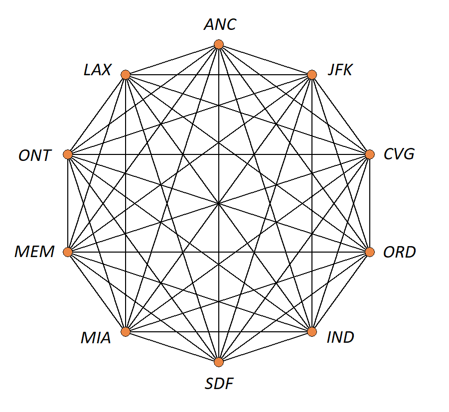
The image shows a graph with vertices representing ten of the busiest airports, by total cargo throughput, in the United States of America. Each vertex is labeled with the International Air Transport Association code for one of the airports, and each edge represents the route between the two airports at the endpoints.
Image credit: Remixer-created derivative of original work "9-simplex graph.png" . The original work has been released into the public domain by its author, Tomruen at English Wikipedia. This applies worldwide.

This table lists each edge with its corresponding weight.

You can download the table as a tab-delimited text file to import the data into a spreadsheet app to sort the list.

You also can view the graph as a map of the routes between the airports at Markus Englund’s Great Circle Map website.

Try to work this out on your own, then confirm that you correctly found the minimal-weight spanning tree by clicking to see the answer below.

Answer

The image shows the edges of the minimal-weight spanning tree in orange. K10-US-airports-spanning-tree

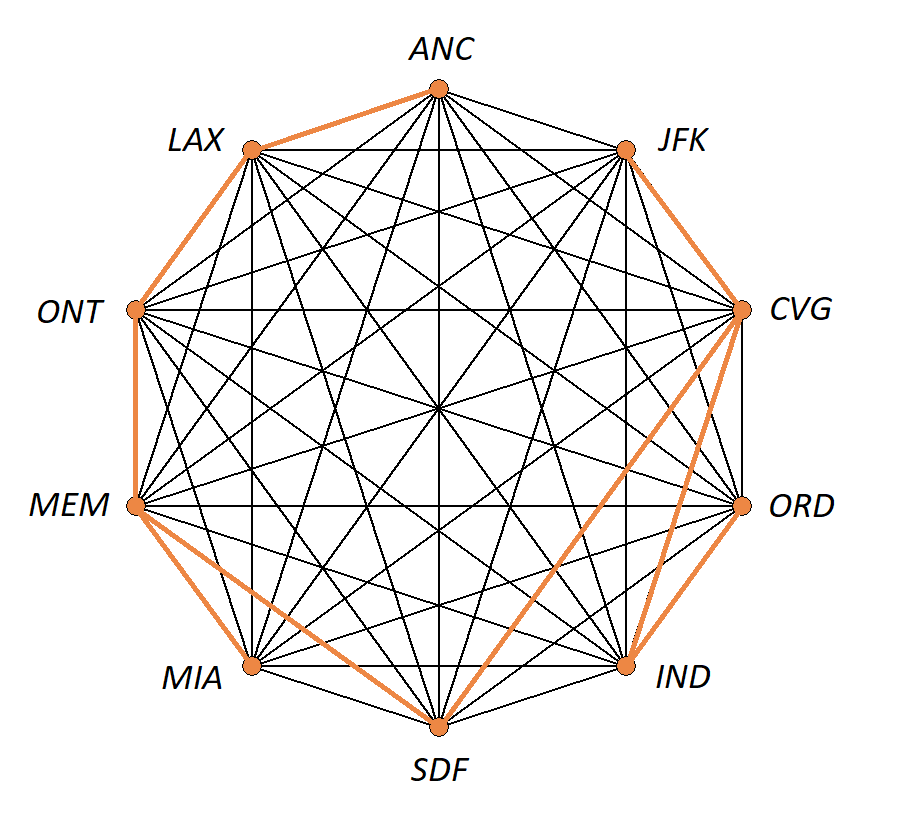
Image credit: Remixer-created derivative of original work "9-simplex graph.png" . The original work has been released into the public domain by its author, Tomruen at English Wikipedia. This applies worldwide.

The table lists the edges of the minimal-weight spanning tree. + +
A map view of the minimal-weight spanning tree can be seen at the Great Circle Map website.

Other Algorithms for Minimal-Weight Spanning Trees

Among the other algorithms that can be used to find a minimal-weight spanning tree are Borůvka’s algorithm and Prim’s algorithm (also known as the DJP algorithm.) You can learn more about these and other algorithms and their history starting with this section of the Wikipedia page about MSTs, as well as the section Historical Notes from Applied Combinatorics by Keller and Trotter.

In 2002, Pettie and Ramachandran published a paper for an optimal minimum spanning tree algorithm.

15.3. Directed Trees

Recall that a tree is defined to be a connected simple graph that contains no cycles. The edges of a tree are undirected.

However, there are applications where it is useful to think of a tree as having directed edges. For that purpose, a directed tree is defined to be a directed graph whose underlying graph is a tree.

15.3.1. Rooted Trees

In some applications of directed trees, you can view the directed tree as if all paths “flow away” from a single vertex. For these applications, the concept of a rooted tree is useful.

The set of rooted trees can be defined recursively as follows.

Basis Step

A single vertex r is a rooted tree. The vertex r is called the root node of this rooted tree.

Recursion

Suppose that you have a nonempty finite set of already-constructed rooted trees (which will be called “old rooted trees” below) such that the following propositions are True:
(1) No vertex appears in more than one of the old rooted trees.
(2) No edge has its two endpoints in two different old rooted trees.
You can construct a new rooted tree by first creating a new root node r that is not a vertex of any of the old rooted trees, and then, for each of the old root nodes, creating a new directed edge from r to that old root node. That is, each new directed edge has initial vertex r and terminal vertex the root node of one of the old rooted trees.

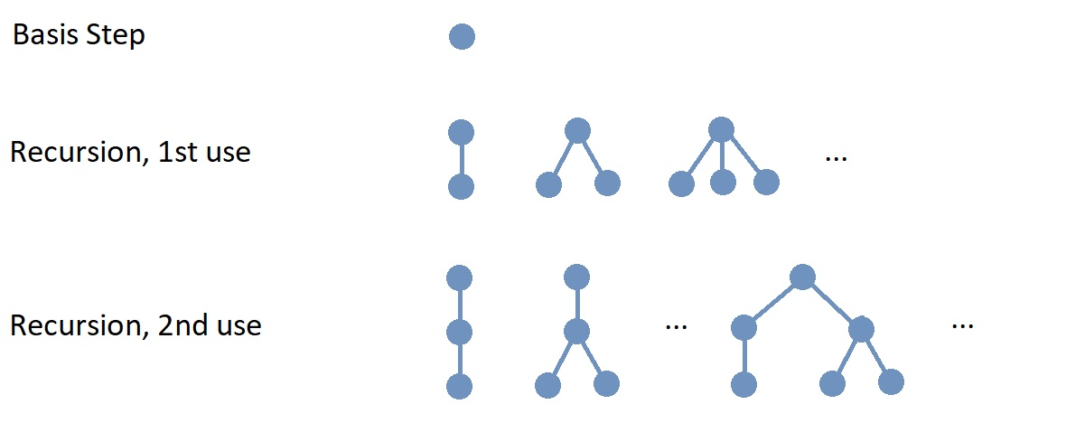
The image shows the basis step and represents, in part, the results of the first and second uses of the recursion step. In the image, the new root node created at each step is drawn at the top of the rooted tree.

Notice that the directed edges of rooted trees are drawn without arrows! Computer scientists usually follow this convention: A rooted tree is drawn with the root node at the top, with all the old root nodes of the previously-constructed rooted trees attached in the Recursion step drawn at the same horizontal level beneath the root node. This convention, along with the recursive definition, ensures that the direction of each directed edge is “down,” so an arrow is not needed to determine the direction of edge.

Notice that if you want to construct just one particular rooted tree, you only need to use the Recursion step finitely-many times. However, at each use of the Recursion step, there is an infinite number of possible rooted trees that can be constructed. Also, to construct all possible rooted trees would require infinitely-many uses of the Recursion step.

Some of the terminology used with rooted trees is borrowed from “family trees,” and other terminology is borrowed from plant science.

The new root node \(r\) added in the Recursion step is called the parent of each of the old root nodes, and each of the old root nodes is called a child of \(r.\) The old root nodes collectively are called the children of \(r.\)
Two or more nodes with the same parent are called siblings.
A node that has one or more children is called an internal node.
A node that has no children is called a leaf. A leaf can also be called an external node.
The depth of node \(v\) in a rooted tree is the length of the shortest path from the root node \(r\) to the node \(v.\) This is also called the level of the node \(v.\)
A level of a rooted tree is the set of all nodes at the same depth. For example, level 1 is the set of all the child nodes of the root node. Level 0 is the set containing only the root node.
The height of a rooted tree is the maximum of the depths of all the nodes in the rooted tree.

The next lemma shows that you can construct any rooted tree without using recursion by instead starting with a tree then replacing all the undirected edges by appropriately directed edges.

Lemma

If \(T\) is a rooted tree, then its underlying graph \(G\) is a tree that has finitely many vertices.
If \(G\) is a tree that has finitely many vertices, then \(G\) is the underlying graph of a rooted tree \(T.\)

Proof outline

First, suppose that \(T\) is a rooted tree. Use strong induction on the number of recursion steps needed to construct the rooted tree to prove that the underlying graph \(G\) must be a simple graph such that for each pair of vertices, there is exactly one path between the vertices. In more detail, for a rooted tree that was constructed using the recursion step only one time, there is only one path between two vertices of the underlying graph: All paths must pass through the root node. For the induction step, any path in the underlying graph of a rooted tree constructed using the recursion step \(k+1\) times will either pass through the new root node or one of the subtree’s root nodes (and the induction hypothesis applies to each underlying graph of the subtrees since they were constructed using fewer than \(k+1\) applications of the recursion step.) Now use the theorem from the first section of the chapter to conclude that \(G\) must be a tree, that is, \(G\) must be a connected simple graph with no cycles. That \(G\) must have finitely many vertices follows from the recursive definition of “rooted tree” since at most finitely many vertices are introduced each time the recursion step is used.

Secondly, suppose that \(G\) is a tree that has finitely many vertices. Use strong induction on the number of vertices to prove that a rooted tree \(T\) can be constructed so that \(G\) is the underlying graph of \(T.\) In more detail, choose any vertex \(r\) of \(G,\) which will become the root node of our rooted tree, then remove \(r\) and any edges incident to \(r\) to create a forest of subtrees \(G_{1}, \, \ldots \, G_{n}\) where \(n\) is the number of trees in the forest. Since each of the subtrees is either a single vertex (which is the basis case for the recursive definition of rooted trees) or a tree that contains fewer vertices than \(G,\) we can apply the induction hypothesis to each of the subtrees to show that each subtree \(G_{i}\) is the underlying graph of a rooted tree \(T_{i}.\) Now apply the recursion step in the definition of rooted trees to reconnect the root nodes of the rooted trees \(T_{1}, \, \ldots \, T_{n}\) to \(r,\) replacing the undirected edges that had been removed by directed edges from \(r\) to each of the root nodes of rooted trees \(T_{1}, \, \ldots \, T_{n}.\) This shows that \(G\) is the underlying graph of a rooted tree. // MKD Aug 15 2025 //It is important to note that, if the direction of the edges matters, you will get a different rooted tree if you choose a different root node (that is, the implied directions of edges will be different even though the underlying undirected graphs will be isomorphic copies of the undirected tree \(G.\)) It is important to note that you will get a different rooted tree if you choose a different root node \(r\) since the directed edges will “flow away” from the root node (That is, the directions of the edges will be different for different choices of root node, but the underlying undirected graph will be the same.)

In summary, the lemma tells you that every rooted tree can be thought of as an adaptation of a tree, where you first select a vertex to be the root node and then replace all the edges of the tree by directed edges that “flow away” from the root node.

15.3.2. Ordered Trees

Notice that in the Recursion step of the definition of rooted tree, the new root node is connected to each of the old root nodes, but since the subtrees' roots are members of a set, the order in which the new root node is connected to the old root nodes is not important. However, in some applications of rooted trees, it is important to note the order in which the new root node is connected to the old root nodes.

For example, in a family tree, you may want to represent a person by the root node of the tree, then represent their offspring by birth order as the child nodes. In this case, the order of the children matters. To do this, you can list the old subtrees as the sequence \(T_{1}, \, \ldots \, T_{n}\) and list the old root nodes as the sequence \(r_{1}, \, \ldots \, r_{n},\) where \(n\) is the number of old subtrees used in the Recursion step.

In this subsection, a recursive definition for ordered trees is presented. This recursive definition takes the order of the indices of the old ordered trees into account when constructing the new ordered tree.
Warning: Many other names for ordered trees appear in various sources, such as ordered rooted tree, rooted plane tree, RP-tree, and decision tree. In fact, some sources even define “rooted tree” to mean what this textbook calls and “ordered tree.”

The set of ordered trees is defined recursively as follows.

Basis Step

A single vertex r is an ordered tree. Vertex r is the root node of this ordered tree.

Recursion

Suppose that you have already constructed the ordered trees in the sequence \(T_{1}, \, \ldots \, T_{n}\) where \(n\) is a positive integer and for each positive integer \(i \leq n,\) the root node of \(T_{i}\) is the vertex \(r_{i}.\)
If both of the propositions
(1) No vertex is in more than one of \(T_{1}, \, \ldots \, T_{n}.\)
(2) No edge has endpoints in two of \(T_{1}, \, \ldots \, T_{n}.\)
are True, then you can construct a new ordered tree by first creating a new root node r that is not a vertex of any of the ordered trees in the sequence \(T_{1}, \, \ldots \, T_{n}\) and then creating \(n\) new directed edges, with one directed edge from \(r\) to each of the old root nodes in the sequence \(r_{1}, \, \ldots \, r_{n},\) in that order. The ordering of the children of the new root node \(r\) corresponds to the increasing order of the subscripts of the old root nodes (which also allows you to use the same ordering for the old ordered trees.)

Ordered trees are usually drawn so that the root node appears at the top of the tree, and for each internal node, the children are drawn in order from left to right.

In summary, an ordered tree can be thought of as a special kind of rooted tree where the children of each internal node are ordered.

15.3.3. Isomorphisms: Rooted Trees and Ordered Trees

As discussed in the Graphs chapter, the definition of isomorphism can be adapted to include one-to-one correspondences between the vertex sets of two graphs that preserve specific features of a graph in addition to the adjacency relationships between vertices. Examples of such features are edge weights, edge directions, vertex colors, or edge colors.

In this subsection, examples are presented to show how the definition of isomorphism can be adapted for rooted trees and ordered trees.

Nonisomorphic Rooted Trees with Isomorphic Underlying Graphs

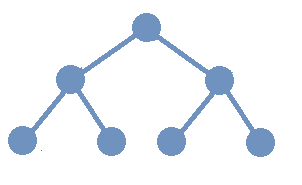
Here is a question for you: In the image, do the two drawings represent graphs or rooted trees? It’s okay if you are not sure how to answer this question. Since rooted trees are usually drawn with edges that do not use arrows to indicate the direction, the drawings are ambiguous, and you would probably need more context to decide whether the drawings represent two undirected graphs or two rooted trees.

Notice that the interpretation also effects whether the two drawings represent isomorphic objects.

Suppose that the drawings are interpreted as undirected graphs. These are isomorphic as undirected graphs, and also isomorphic as trees, since redrawing the graph on the left as the one on the right does not change the adjacency relationships of the vertices.
Suppose that the drawings are interpreted as rooted trees. The adjacency relationships are the same, but the direction of the edge with endpoints \(A\) and \(B\) depends on whether \(A\) or \(B\) is chosen as the root node. The underlying graphs with undirected edges are isomorphic, but the rooted trees are not isomorphic.

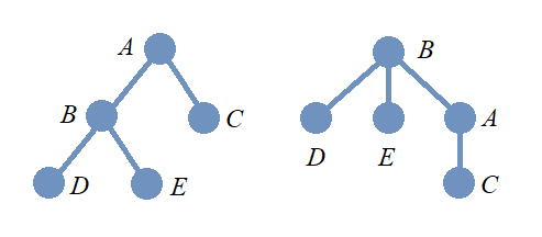
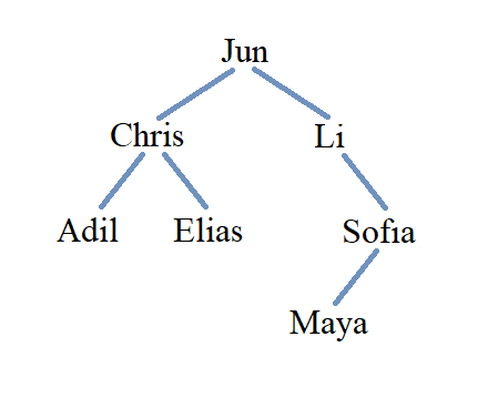
Nonisomorphic Ordered Trees that are Isomorphic Rooted Trees

In the image, two rooted trees are shown. The two rooted trees are isomorphic as rooted trees since the order of the children of the root node does not matter. However, these two rooted trees are not isomorphic as ordered trees since the corresponding children are not in the same order in each rooted tree.

It may be helpful to think of each of the two ordered trees as “telling a story” about a family.

On the left, a parent has three children, and the oldest child has three children, the middle child has no children, and the youngest child has one child.
On the right, a parent has three children, and the oldest child has no children, the middle child has three children, and the youngest child has one child.

In general, ordered trees are isomorphic if and only if they tell the same story about the families, so these two are not isomorphic as ordered trees. On the other hand, they are isomorphic as rooted trees because they tell the same story when the birth order of the children at level 1 is ignored: A parent has three children, of whom one has three children, another one has one child, and yet another one has no children.

15.4. Binary Trees

As mentioned near the beginning of this chapter, much of the terminology related to trees is not standardized. The definitions in this section use terminology consistent with Handbook of Graph Theory, Second Edition, but information on alternative definitions is also stated.

For any positive integer \(m,\) an m-ary tree is defined to be an ordered tree in which each internal node has at most \(m\) children.
Some sources define m-ary tree to be a rooted tree instead of an ordered tree.

A binary tree is a 2-ary tree, or more simply, an ordered tree in which each internal node has at most two children. In a binary tree, the root node is the parent of at most two subtrees \(T_{1},\) called the left subtree, and \(T_{2},\) called the right subtree. Notice that in the context of binary trees, it is allowable for either or both of the subtrees to be absent (that is, empty).
Some sources allow a binary tree to be “empty,” in the sense that it has no vertices or edges. An “empty binary tree” is not an ordered tree as defined above since it has no root node. However, an empty binary tree is useful in computer science applications. For example, when implementing binary trees as data structures, an empty binary subtree corresponds to by a null pointer (or null reference); a leaf node of a binary tree can be recognized as a node whose left child and right child pointers/references are both null.

A complete binary tree is a binary tree in which every internal node has exactly 2 children and all leaves are at the same level.
Some sources use either “perfect binary tree” or “full binary trees” to describe this type of binary tree and use the phrase “complete binary tree” to describe something else.

A binary tree is called balanced if for every vertex \(v,\) the number of vertices in the left subtree of \(v\) and the number of vertices in the right subtree of \(v\) differ by at most one.
Some sources define a binary tree of height \(h\) to be balanced if each leaf is at either level \(h\) or level \(h − 1.\)

15.4.1. Tree Traversal Algorithms for Binary Trees

In many applications of binary trees, it is necessary to visit every node. The process of visiting every node is called tree traversal. In this subsection, you will learn about three commonly-used algorithms for tree traversal.

The three traversal algorithms can be described recursively as follows.

Preorder traversal: First, visit the root node. Secondly, visit each node in the root node’s left subtree using preorder traversal. Finally, visit each node in the root node’s right subtree using preorder traversal.
Inorder traversal: First, visit each node in the root node’s left subtree using inorder traversal. Secondly, visit the root node. Finally, visit each node in the root node’s right subtree using preorder traversal.
Postorder traversal: First, visit each node in the root node’s left subtree using postorder traversal. Secondly, visit each node in the root node’s right subtree using postorder traversal. Finally, visit the root node.

For each of these three traversal algorithms, the Base Step for the recursion is applied to a binary tree that has only one node (a root node that has empty left and right subtrees), and you visit just that one node.
Some sources use hyphens in the written names of these traversal algorithms, so list them as pre-order, in-order, and post-order traversal.

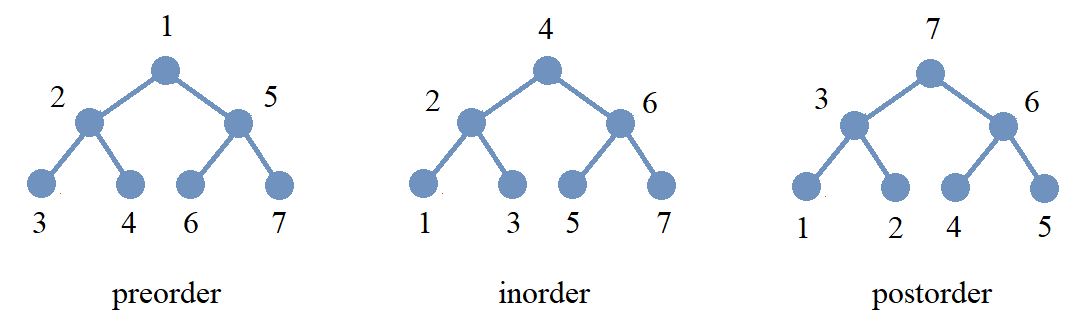
The image displays the same binary tree with its nodes being “counted off” using each of these three traversal algorithms.

You may find the interactive demonstration at this Wikipedia page useful to understanding these three traversal algorithms.

15.4.2. Binary Search Trees

Define a key to be an element of a set that has a total ordering. For example, keys could be integers ordered using the usual \(\leq\) relation. As another example, keys could be strings ordered alphabetically. In general, keys could be any type of data that can be totally ordered.

A binary search tree (BST) is a binary tree where each vertex is assigned a key in such a way that that if key \(k\) is assigned to vertex \(v\) then both of the following are True.

the key \(k\) is greater than each key assigned to a vertex in the left subtree of \(v,\) and
the key \(k\) is less than each key assigned to a vertex in the right subtree of \(v.\)

If you are given a list (or an array) of keys, a binary search tree can be used to sort the keys and then quickly search for a key. An advantage of binary search trees is that it is much easier and faster to maintain the sort order if you need to insert new keys than it would be to insert the same keys into a sorted list (or an array) of keys.

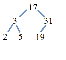
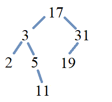
Example 2 - Constructing a Binary Search Tree

First, let’s construct a binary search tree from the list of keys \( \left[ 17, 3, 5, 31, 2 \right .\)]

The first key in the list, \(17,\) is assigned to the root node.
The next key, \(3,\) is less than the key \(17\) at the root node, so \(3\) is assigned to the left child of the root node.
The next key, \(5,\) is less than the key \(17\) at the root node, so \(5\) must be assigned to some node in the left subtree.
- Since \(5\) is greater than the key \(3\) at the left subtree’s root, \(5\) is assigned to the right child of the left subtree’s root.
The next key, \(31,\) is greater than the key \(17\) at the root node, so \(31\) is assigned to the right child of the root node.
The last key, \(2,\) is less than the key \(17\) at the root node, so \(2\) must be assigned to some node in the left subtree.
- Since \(2\) is greater than \(3,\) \(2\) is assigned to the left child of of the left subtree’s root.

The following animation illustrates the construction of this binary search tree.

Now, let’s search for some keys. If a key is not already present, it will be inserted in the correct position.

Consider the key \(5.\)

\(5\) is less than the key at the root node, which is \(17.\) If \(5\) is in this BST, it must be in the left subtree, so continue searching from there.
\(5\) is greater than the key at the left subtree’s root node, which is \(3.\) If \(5\) is in this BST, it must be in the right subtree of this node, so continue searching from there.
\(5\) is equal to the key at the subtree’s root node, so we have found this key!

Now consider the key \(19\) which was not included in the original list.

\(19\) is greater than the key at the root node, which is \(17.\) If \(19\) is in this BST, it must be in the right subtree, so continue searching from there.
\(19\) is less than the key at the right subtree’s root node, which is \(31.\) If \(19\) is in this BST, it must be in the left subtree of this node, so continue searching from there.
This subtree is empty, so insert a new root node for this subtree and assign the key \(19\) to this new node.

The following image shows the modified BST with the new key \(19\) inserted in the correct position.

You Try

Locate the correct position of the new node when the key \(11\) is inserted in the previously modified BST.

Answer

The key \(11\) is assigned to the right child of the node that has the key \(5.\) Click here to see an image of the BST with \(11\) assigned to the new node.

Constructing a binary search trees from a list can serve two purposes. First, as shown in the preceding example, it is quicker to search for a key in the binary search tree because, in the best case scenario when the tree is balanced, the number of keys is halved with each iteration of the search. Secondly, the original list can be sorted by performing an inorder traversal of the binary search tree.

Exercise - Traversing a Binary Search Tree

Consider the binary search tree with integer keys that was the solution in the “You Try” section of the previous example.

List the keys of the binary search tree using each of preorder, inorder, and postorder traversal to visit all nodes of the binary search tree.

Answer

Preorder: \( \left[ 17, 3, 2, 5, 11, 31, 19 \right .\)]
Inorder: \( \left[ 2, 3, 5, 11, 17, 19, 31 \right .\)]
Preorder: \( \left[ 2, 11, 5, 3, 19, 31, 17 \right .\)]

Here is another exercise for you to try.

Check Your Understanding

Consider the following list of names, which will be used as alphabetically-ordered keys. \[ \left[ \text{Jun, Li, Chris, Elias, Sofia, Adil, Maya} \right] \]

First, construct and draw the binary search tree for this list of keys.

Answer

Click here to see an image of the BST.

Next, write down the three lists you get by using preorder, inorder, and postorder traversals to visit all nodes of the binary search tree.

Answer

Preorder: [ Jun, Chris, Adil, Elias, Li, Sofia, Maya ]
Inorder: [ Adil, Chris, Elias, Jun, Li, Maya, Sofia ]
Preorder: [ Adil, Elias, Chris, Maya, Sofia, Li, Jun ]

15.4.3. Expression Trees and Polish Notation

In the 1920’s, the Polish logician Jan Łukasiewicz created a notational format for writing logical well-formed formulas that does not use any parentheses: Instead of writing logical operator symbols (like \(\land\) and \(\lor\)) between two previously-constructed wffs, Łukasiewicz placed operator symbols in front of those wffs, which makes the use of parentheses completely unnecessary! Today, notation that is based on Łukasiewicz’s original notation is called either Polish notation or prefix notation and is applied to both arithmetic/algebraic formulas and logical formulas.

There is also the Reverse Polish notation, also called postfix notation, where the operator symbol is placed after its operands. The “usual” notation where the operator symbol is placed between the two operands is called infix notation.

Example 3 - Polish and Reverse Polish notation

Consider the following algebraic expression, written in infix notation. \[ 3 \cdot x - 5 \]

The Polish notation (prefix notation) for the same expression is \[ - \, \cdot \, 3 \, x \, 5 \] and the Reverse Polish notation (postfix notation) for the expression is \[ 3 \, x \, \cdot \, 5 \, - \]

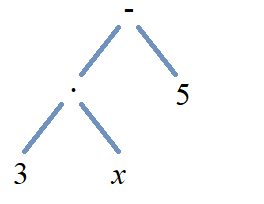
You can use binary trees and tree traversal to make it easier to switch between these three notations. Define an expression tree to be a binary tree where each leaf is labeled by either a numeral or a variable symbol, and where each internal node is labeled by an operator symbol. The expression tree for the infix notation \(3 \cdot x - 5\) is shown. Notice that in the expression tree for \(3 \cdot x - 5,\) the root node corresponds to the “last” operation you would perform and the subtrees correspond to the previously-constructed expressions \(3 \cdot x\) and \(5.\) Also notice that, in the earlier example, the order of the symbols for the infix expression corresponds to the inorder traversal of the expression tree. It is an exercise for you to confirm that the order of the symbols in the Polish notation expression corresponds to the preorder traversal of the expression tree, and that the Reverse Polish notation expression corresponds to the postorder traversal of the expression tree.

Example 4 - Building And Traversing An Expression Tree

Consider the arithmetic expression. \[ 5 + 7 \times - 3 - 8 \div 2 \] Recall that it is not correct to evaluate this left-to-right; instead you need to use the order of operations, which is equivalent to evaluating the following expression that results after inserting parentheses. \[ (5 + (7 \times (- 3))) - (8 \div 2) \] From this second expression, you can see that the expression tree will have the minus sign at the root and subtrees that represent \((5 + (7 \times (- 3)))\) and \((8 \div 2).\) Continuing recursively, the subtree for \((5 + (7 \times (- 3)))\) will have the plus sign at its root and subtrees that represent \(5\) and \((7 \times (- 3)),\) and the subtree for \((8 \div 2)\) will have the division sign at its root node and subtrees that represent \(8\) and \(2.\) Continue recursively until all symbols have been placed at a node.

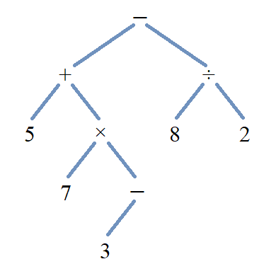
The image displays a drawing of the expression tree for \((5 + (7 \times (- 3))) - (8 \div 2)\). Notice that the negative sign labels a node with only one child, which is treated as the left child (but as the right child for inorder traversal. )

Next, you can use each of the traversal methods to create the Polish (prefix), infix, and Reverse Polish (postfix) expressions.

\(\text{prefix: } \ - \, + \, 5 \, \times \, 7 \, - \, 3 \, \div \, 8 \; 2 \)

\(\text{infix: } \ 5 \, + \, 7 \, \times \, - \, 3 \, - \, 8 \, \div \, 2 \)

\(\text{postfix:} \ 5 \, 7 \, 3 \, - \, \times \, + \, 8 \; 2 \, \div \, - \)

You can see another example of how to construct expression trees, using Reverse Polish notation and a stack, at this Wikipedia page.

15.4.4. Isomorphisms: Binary Trees

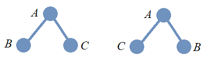
In the image, two binary trees are shown. As binary trees are ordered trees, it should be clear that these cannot be isomorphic as binary trees because the order of the left and right children of the root node in the two trees are different.

15.5. Additional Topics To Be Added Later

Algorithms for Depth- and breadth-first traversals