9. Relations
CAUTION - CHAPTER UNDER CONSTRUCTION!
NOTICE: If you are NOT enrolled in the CSC 230 course that I teach at SFSU, you probably are looking for the “public version” of the book, which I only update between semesters. The version you are looking at now is the “CSC230 version” of the book, which I will be updating throughout the semester.
This chapter was last updated on March 16, 2026.
Inserted content on the so-called “Chinese Remainder Theorem.”
Inserted proof of the Division Algorithm using the Well-Ordering Principle.
Revised the sections/subsections on partial orders, well-ordering, and modular arithmetic.
Made other minor revisions and fixed typos.
Relations are used to describe an association of data.
For example, imagine a university database of students. The database needs to have a record for each student, and the student’s record needs to include fields for the student’s name(s), the unique student ID number for the student, the student’s current status, a list of courses that the student has enrolled in or has completed (along with the grade earned in each completed course,) and possibly other data associated with the student. One way to visualize the database is as a two-dimensional table, similar to a spreadsheet worksheet, where each row corresponds to a record and each column corresponds to a field; each row can be treated as an ordered \(n\)-tuple, where \(n\) is the number of fields.
In this chapter, you will learn about the formal definition of relation, operations and properties of relations. You will also learn about some special types of relations, namely partial orderings and equivalence relations. As a special case of equivalence relations, you will learn about congruence relations of integers as well as modular arithmetic.
Key terms and concepts covered in this chapter:
-
Relations
-
Properties of relations (reflexivity, symmetry, transitivity, and other properties)
-
Equivalence relations
-
Equivalence classes
-
-
Modular arithmetic
-
Congruences
-
-
Partial orders
-
Well orderings
9.1. Definition of Relation
Informally, a relation on two or more sets is an association between elements of those sets.
Formally, a relation is a subset of a Cartesian product of two or more sets.
For simplicity, it is assumed in this textbook that the number of sets used to form the Cartesian product is finite. It
is
possible to define relations as subsets of a Cartesian product of infinitely many sets, in which case the elements of the relation are infinite sequences.
Here are several examples of relations.
Notice that for any sets \(A_{1}, \, A_{2}, \, \ldots \, A_{n},\) where \(n \geq 2\) is a natural number, we always have the following two relations:
-
\(\emptyset,\) called the empty relation. This relation is also called the void relation and trivial relation in other sources.
-
\(A_{1} \times A_{2} \times \cdots \times A_{n},\) called the universal relation.
9.2. Binary Relations on a Single Set
In many cases, the two domains of a binary relation are the same set; for example, the relation may involve comparing two elements of a set S in some way. In this case, the domain \(S\) is mentioned only once: A binary relation on set S is any subset \(R\) of the cartesian product \(S \times S\), that is, \(R \subseteq S \times S.\)
In the case of a binary relation on \(S,\) we often write \(aRb\) to mean the same thing as \((a,b) \in R.\) This notation may make more sense after reading the following example.
9.2.1. Operations on Binary Relations on a Set
Given binary relations \(Q\) and \(R\) on a set \(S,\) we can define several other relations in terms of \(Q\) and \(R.\) These operations are likely familiar to you as operations on functions but they also work for binary relations on a single set.
-
The inverse of \(R\) is the relation \(R^{-1} = \{ (b,a) \, | \, (a,b) \in R \}.\)
-
The composition of Q and R is \(R \circ Q = \{ (a,c) \, | \, (a,b) \in Q \land (b,c) \in R \}.\)
-
The n th power of \(R\) is defined recursively for all \(n \in \mathbb{N}\) as follows.
-
\(R^{0} = \mathbf{id}_S\)
-
\(R^{k+1} = R \circ R^{k}\) for natural numbers \(k > 0.\)
The recursion step uses \(k\) instead of \(n\) in preparation for the type of arguments used in the chapter on proof by mathematical induction.
-
Building on the \(n\)th powers of \(R,\) we can define two relations.
-
\(R^{+}\) is the relation \(\{ (a,b) \in S \times S \, | \, (a,b) \in R^{k} \text{ for some positive integer } k \}.\) That is, \(R^{+}\) is the union of all the positive \(n\)th powers of \(R.\)
-
\(R^{*}\) is the relation \(\{ (a,b) \in S \times S \, | \, (a,b) \in R^{k} \text{ for some natural number } k \}.\) That is, \(R^{*}\) is the union of all the natural number \(n\)th powers of \(R.\)
Notice that \(R^{*} = \mathbf{id}_S \cup R^{+}.\)
9.2.2. Properties of Binary Relations on a Set
In this subsection we define five properties that a relation may satisfy.
The following theorem can make it easier to determine when a relationship has each of the five properties. The proof of the theorem is an exercise.
9.2.3. Closures of Binary Relations with Respect to a Property
For each of the properties reflexivity, symmetry, and transitivity, we define the closure with respect to the property of a relation \(R\) as follows: The closure is the smallest relation that has the property and includes all the elements of \(R.\) That is, you start with \(R\) and try to insert in just enough ordered pairs, if any are needed, to make sure that the new relation has the desired property.
The following theorem justifies that the reflexive closure, symmetric closure, and transitive closure exist for any relation \(R.\) The proof of the theorem is an exercise.
Notice that we can also define the reflexive and transitive closure of a relation \(R\) as the relation \(R^{*},\) which is the reflexive closure of the transitive closure of \(R.\)
However, for some properties, the closure of a relation \(R\) with respect to the property may not exist!
9.3. Equivalence Relations
A binary relation \(R\) on a set \(S\) is called an equivalence relation on \(S\) if \(R\) is reflexive, symmetric, and transitive.
A first example of an equivalence relation is the diagonal, that is, the equality relation. Another example is given below.
Given an equivalence relation \(R\) on the set \(S\) and an element \(x \in S,\) we define the equivalence class of \(x\) to be \([ x ]_{R} = \{ y \in S \, | \, (x,y) \in R \}.\)
9.4. Order Relations on a Set
It is often useful to be able to compare elements of a set, based on some key property. In this subsection, several examples of such order relations will be discussed.
9.4.1. Partial Orderings
A binary relation \(R\) on a set \(S\) is called a partial order on \(S\) if \(R\) is reflexive, antisymmetric, and transitive.
For any set \(S,\) each of the relations \(\subseteq\) and \(\subset\) is a partial order on \(\mathcal{P}(S),\) the power set of \(S.\)
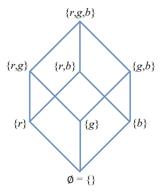
As an example, for the set \(S = \{ r, g, b \},\) the image shows a Hasse diagram that represents the \(\subset\) relation on the power set \(\mathcal{P}(S).\) Notice that each line segment in the Hasse diagram connects a first subset of \(S\) to a second subset of \(S\) that is “immediately above” the first subset in the following sense: Each member of the first subset is also a member of the second subset, but the second subset has one additional member. In the Hasse diagram, two different subsets \(A\) and \(B\) satisfy \(A \subset B\) if and only if there is a “path up” from \(A\) to \(B\) that uses one or more of the line segments.
Total Orderings
A total ordering of a set \(S\) is a partial order \(R\) on \(S\) that has the additional property \((\forall x \in S)(\forall y \in S)(xRy \lor yRx).\)
Well-Orderings
A well-ordering of a set \(S\) is a total ordering \(R\) on \(S\) that has the additional property that every nonempty subset of \(S\) contains a least element with respect to the order relation.
One of the most important examples of a well-ordering in mathematics is the relation \(\leq\) on the set of natural numbers \(\mathbb{N}.\)
In the Remix, the Well-Ordering Principle is treated as an axiom, a statement that is assumed to be True about the set of natural numbers.
The Well-Ordering Principle may seem like an “obviously True” statement. To understand why mathematicians would make it clear that they are assuming that this principle is True is to understand what “infinity” means.
-
First, suppose that you are told that the subset \(A\) of \(\mathbb{N}\) contains the element 10. You can use a brute‑force method to determine the least element of \(A:\) Just ask the following sequence of 10 questions, in the order shown. \[ \text{“Is 0 in \(A?,\)” “Is 1 in \(A?,\)” \(\ldots\), “Is 9 in \(A?\)”} \] If the answer is “No” to all 10 of these questions, then 10 itself is the least element in \(A\), otherwise, the least number in \(A\) is the first value of \(k\) for which the answer to the question “Is \(k\) in \(A?\)” is “Yes.”
-
Next, suppose that you are given a new set \(S\) and told that the number \(10^{10^{10^{10^{10}}}}\) is in \(S.\) You again could try to use the brute‑force method of asking the sequence of \(10^{10^{10^{10^{10}}}}\) questions: \[ \text{“Is 0 in \(S?,\)” “Is 1 in \(S?,\)” \(\ldots\), “Is \(\left( 10^{10^{10^{10^{10}}}}-1 \right)\) in \(S?\)”} \] but even if it took only 1 nanosecond to ask and answer each question, the integer \(10^{10^{10^{10^{10}}}}\) is greater than the number of nanoseconds estimated for our universe to reach its final energy state! That is, it is possible that the answer to one of these questions is “Yes” but that you would never be able to ask that question before the universe ends! Notice that you can use formal logic to justify that either the answers to all of those questions would be “No” or that at least one of the questions would have the answer “Yes” — asking the sequence of questions would determine the least element in \(S\) if you had time to ask enough of the questions, but you (and humanity itself) may not have that much time. For this reason, mathematicians assume that the least element of the set \(S\) exists.
Notice that a “timeless being” could know all the answers.
Greatest Common Divisors section in progress
In this subsection, we will use the Well-Ordering Principle to prove a theorem that will be used later in the chapter.
Suppose that \(a\) and \(b\) are two positive integers. The greatest common divisor of \(a\) and \(b,\) abbreviated as gcd, is the greatest integer that divides both integers \(a\) and \(b.\) That is, the gcd of \(a\) and \(b\) is a divisor of both \(a\) and \(b,\) and is divisible by any other positive divisor of \(a\) and \(b.\)
9.5. Modular Arithmetic (Revision in Progress!)
Let \(m\) stand for some positive integer constant that is greater than 1. The relation congruence modulo \(m\) is defined to be \[\{ (a, b) \in \mathbb{Z} \times \mathbb{Z} \, : \, m \text{ divides } (a-b) \}.\] The symbol \(\equiv_{m}\) is used to represent congruence modulo \(m\), so \[a \equiv_{m} b \text{ if and only if } m \text{ divides } (a-b).\]
As an example, \(13 \equiv_{3} 7\) because \(3\) divides \(13-7.\) Another way to see that \(13 \equiv_{3} 7\) is to notice that both \(13\) and \(7\) leave a remainder of \(1\) when divided by \(3\) using integer long division.
Notice that the relation \(\equiv_{2}\) is the same as the parity relation discussed in an example earlier in this chapter. As discussed in that example, \(\equiv_{2}\) is an equivalence relation. In fact, for each positive integer constant \(m\) that is greater than 1, the relation \(\equiv_{m}\) is an equivalence relation.
We can also do “arithmetic” directly with the equivalence classes of the \(\equiv_{m}\) relation. The following example may make this more clear.
You likely learned, when you were quite young, that some integers are called "even" and other integers are called "odd."
Notice that every integer is either even or odd but not both, which means that the set \[\{ \text{the set of all even integers}, \, \text{the set of all odd integers} \}\] or more formally \[\{ \{ \ldots, -4, -2, 0, 2, 4, \ldots \}, \, \{ \ldots, -3, -1, 1, 3, \ldots \} \}\]forms a partition of the set \(\mathbb{Z}\) of integers. This partition corresponds to the relation \(\equiv_{2},\) that is, congruence modulo 2. The set of all even numbers is the equivalence class \([ 0 ]_{\equiv_{2}}\) and the set of all odd numbers is the equivalence class \([ 1 ]_{\equiv_{2}}.\)
You may have learned how to do arithmetic with "Even" and "Odd," too, as shown in the tables.
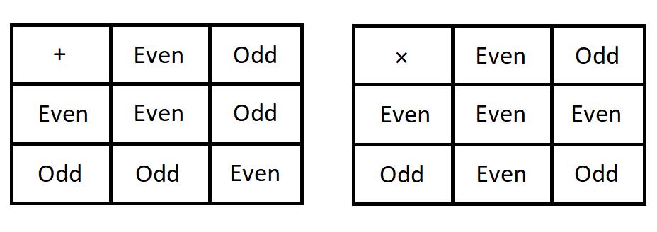
When you did arithmetic with "Even" and "Odd," you were really doing arithmetic with the equivalence classes \([ 0 ]_{\equiv_{2}}\) and \([ 1 ]_{\equiv_{2}}.\) For example, it will not matter which two odd numbers you add, the result must be even because the two numbers were odd. You can just do the operations on the remainders that you get after dividing by 2, which corresponds to adding the equivalence classes: \([ 1 ]_{\equiv_{2}} + [ 1 ]_{\equiv_{2}} = [ 1+1 ]_{\equiv_{2}} = [ 2 ]_{\equiv_{2}} = [ 0 ]_{\equiv_{2}}\) where the last equality is True because \(2\) and \(0\) belong to the same equivalence class (that is, they are both even numbers.)
The following theorem proves that you can do addition and multiplication with the remainders (or, what amounts to the same thing, the equivalence classes) in the same way as was done with Evens and Odds in the previous example for the relation \(\equiv_{m},\) where \(m\) can be any integer greater than 1.
For example, we can write \(9 + 5 \equiv_{12} 2\) (This is an example of "clock arithmetic" using a 12-hour clock: 5 hours after 9 o’clock will be 2 o’clock.)
9.6. Sunzi’s Method (The “Chinese Remainder Theorem”) section in progress
In this section, you will learn a method for solving a simultaneous system of linear congruences that has application to encryption.
This method is based on the solution of a problem from 孫子算經 (“The Mathematical Classic of Sun Zi”) which was written sometime during the 3rd, 4th, or 5th century AD. The box below presents an English translation, using Google Translate, of the original problem.
There is an unknown number of objects. When counted in groups of three, two remain; when counted in groups of five, three remain; when counted in groups of seven, two remain. How many objects are there?
This can be stated using modular arithmetic notation as follows.
Solve the following system of congruences. \begin{equation} \begin{aligned} n \equiv_{3} 2 \\ n \equiv_{5} 3 \\ n \equiv_{7} 2 \end{aligned} \end{equation}
You can verify that one solution is \(23,\) but in this section, we will build up a method for finding all solutions of any such system of congruences.
9.6.1. Step 1
First notice that one solution \(n\) of the simultaneous system \begin{equation} \begin{aligned} n \equiv_{3} 0 \\ n \equiv_{5} 0 \\ n \equiv_{7} 0 \end{aligned} \end{equation} is the least common multiple of \(3,\) \(5,\) and \(7,\) which is \(105.\) That is, dividing \(105\) by each of those primes leaves a remainder of \(0.\)
Furthermore, notice that each integer multiple \(105 \cdot k\) is a solution as well. This shows that the set of all solutions to this system is \(\{ 105 \cdot k \, : \, k \in \mathbb{Z} \}.\)
9.6.2. Step 2a
Next, we will find one solution of the simultaneous system \begin{equation} \begin{aligned} n \equiv_{3} 1 \\ n \equiv_{5} 0 \\ n \equiv_{7} 0 \end{aligned} \end{equation}
Notice that any solution must be a multiple of \(5 \cdot 7 = 35\) that leaves a remainder of \(1\) when it is divided by \(3.\) For now, we can just use “trial-and-error” to find a solution.
\(0 \equiv_{3} 0\) since \(0 = 0 \cdot 3 + 0\)
\(35 \equiv_{3} 2\) since \(35 = 11 \cdot 3 + 2\)
\(70 \equiv_{3} 1\) since \(35 = 23 \cdot 3 + 1\)
Notice that the remainders will repeat periodically for the multiples of \(35.\)
So one solution of this system of congruences is \(70.\)
9.6.3. Step 2b
Next, find one solution of the simultaneous system \begin{equation} \begin{aligned} n \equiv_{3} 0 \\ n \equiv_{5} 1 \\ n \equiv_{7} 0 \end{aligned} \end{equation}
Notice that any solution must be a multiple of \(3 \cdot 7 = 21\) that leaves a remainder of \(1\) when it is divided by \(5.\) Again, we can just use “trial-and-error” to find a solution.
\(0 \equiv_{5} 0\) since \(0 = 0 \cdot 5 + 0\)
\(21 \equiv_{5} 1\) since \(21 = 4 \cdot 5 + 1\)
So one solution of this system of congruences is \(21.\)
9.6.4. Step 2c
And now we find one solution of the simultaneous system \begin{equation} \begin{aligned} n \equiv_{3} 0 \\ n \equiv_{5} 0 \\ n \equiv_{7} 1 \end{aligned} \end{equation}
Any solution must be a multiple of \(3 \cdot 5 = 15\) that leaves a remainder of \(1\) when it is divided by \(7.\) Once again, we use “trial-and-error” to find a solution.
\(0 \equiv_{7} 0\) since \(0 = 0 \cdot 7 + 0\)
\(15 \equiv_{7} 1\) since \(15 = 2 \cdot 7 + 1\)
So one solution of this system of congruences is \(15.\)
9.6.5. Step 3
We can now find all solutions of the simultaneous system \begin{equation} \begin{aligned} n \equiv_{3} 2 \\ n \equiv_{5} 3 \\ n \equiv_{7} 2 \end{aligned} \end{equation}
Each solution must be of the form \((2 \cdot 70) + (3 \cdot 21) + (2 \cdot 15) + (105 \cdot k)\) where \(k\) can be any integer.
That is, \(233 + 105 \cdot k\) is a solution for each integer \(k.\) Notice that \(23\) corresponds to \(k = -2.\)