17. Appendix: Library of Functions
NOTICE: If you are enrolled in the CSC 230 course that I teach at SFSU, you need to use the “CSC230 version” of the book, which I will be updating throughout the semester. The version you are looking at now is the “public version” of the book that will not be updated again before the start of June 2026.
This chapter was last updated on August 24, 2025.
repaired some typos
Recall that for any function,
-
the domain is the given set of input values for the function,
-
the codomain is a given set that contains all possible output values (but may contain other values that are not outputs, too), and
-
the range is the set that contains only the output values of the function.
Functions can in many cases be visualized graphically, for example when mapping from the real line, \(\mathbb{R}\) to the real line, such maps are viewed on a Cartesian plane.
17.1. Polynomial Functions
A polynomial is an algebraic expression of the form \(a_{n}x^{n} + a_{n-1}x^{n-1} + \ldots + a_{1}x^{1} + a_{0}\), that is, \(\sum\limits_{i=0}^{n}a_{i}x^{i}\), where n is a natural number, x is a variable, and \(a_{n}, a_{n-1}, \ldots, a_{1}, a_{0}\) are real numbers. Examples of such expressions are
-
7, a constant,
-
\(2x + 7\), a linear polynomial,
-
\(3x^{2} + 2x + 7\), a quadratic polynomial.
A polynomial can be evaluated by substituting a number for each occurence of x . For example, if we substitute \(-1\) for x in each of the three polynomials above, we get
-
7 evaluated at \(x = -1\) is 7,
-
\(2x + 7\) evaluated at \(x = -1\) is \(2 \cdot (-1) + 7 = 5\),
-
\(3x^{2} + 2x + 7\) evaluated at \(x = -1\) is \(3 \cdot (-1)^{2} + 2 \cdot (-1) + 7 = 8.\)
In this way, every polynomial can be used to define a corresponding polynomial function with domain \(\mathbb{R}\) and codomain \(\mathbb{R}.\)
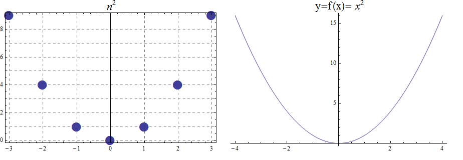
17.1.1. Quadratic Function
The function \(f(x) =x^2\), denotes the association \((a,b) =(x, x^2)\) with \(f : \mathbb{R} \rightarrow \mathbb{R}\). We notice that the range is the set of real numbers \([0, \infty)= \mathbb{R}^{+}\). The function is not invertible, since it is not injective. For example, we have both \(f(-3) =9\) and \(f(3)=9\). With \(f : \mathbb{Z} \rightarrow \mathbb{Z}\) notice that the range is now \(\mathbb{N}\)
\begin{array}{lccccccccccc} & x & -5 & -4 & -3 & -2 & -1 & 0 & 1 & 2 & 3 & 4 & 5 \\ & x^2 & 25 & 16 & 9 & 4 & 1 & 0 & 1 & 4 & 9 & 16 & 25 \end{array}
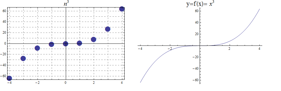
17.1.2. The Cubic function
The function \(f(x) =x^3\), denotes the association \((a,b) =(x, x^3)\) with \(f : \mathbb{R} \rightarrow \mathbb{R}\). Also, we notice that the range is the set of all real numbers \((- \infty , \infty)=\mathbb{R}\). The function is bijective and so invertible. With \(f : \mathbb{Z} \rightarrow \mathbb{Z}\), notice that the range, in addition to domain, is also \(\mathbb{Z}\)
\begin{array}{llcccccccccl} & x & -5 & -4 & -3 & -2 & -1 & 0 & 1 & 2 & 3 & 4 & 5 \\ & x^3 & -125 & -64 & -27 & -8 & -1 & 0 & 1 & 8 & 27 & 64 & 125 \end{array}
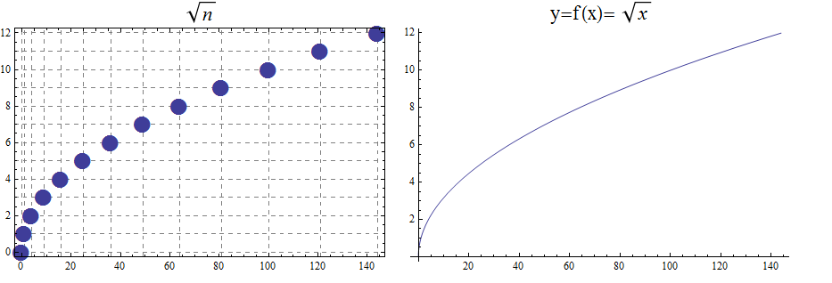
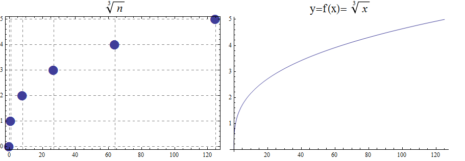
17.1.3. The Square Root and Cube Root Functions
For the purposes of completeness and for comparing how fast functions \(f(x)\) grow for large x, we present the inverse of the functions \(f(x)= x^2\) and \(f(x)= x^3\), when \(f(x):\mathbb{R}+→\mathbb{R}+\). Respectively, the functions\( f(x)=\sqrt{x}\) and \(f(x)= \) \$root(3)(x)\$.
\begin{array}{lcccccccccclll} & x & 0 & 1 & 4 & 9 & 16 & 25 & 36 & 49 & 64 & 81 & 100 & 121 & 144 \\ & \sqrt{x} & 0 & 1 & 2 & 3 & 4 & 5 & 6 & 7 & 8 & 9 & 10 & 11 & 12 \end{array}
\begin{array}{lcccccl} & x & 0 & 1 & 8 & 27 & 64 & 125 \\ & \sqrt[3]{x} & 0 & 1 & 2 & 3 & 4 & 5 \end{array}
17.2. Exponential and Logarithmic Functions
We begin by summarizing important properties of exponentials.
17.2.1. Exponential Functions
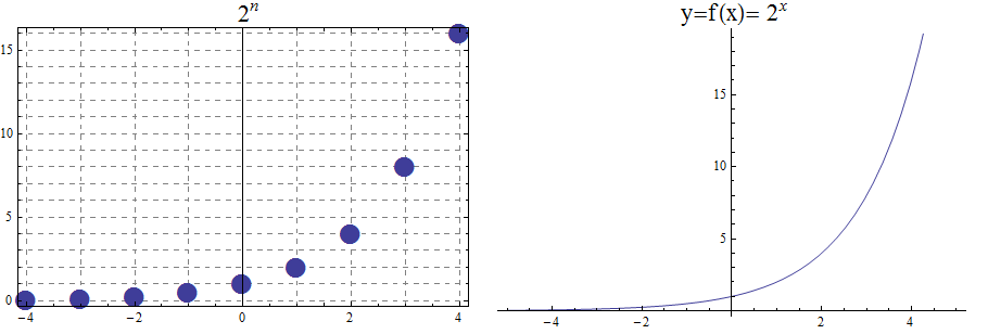
Exponential functions are of the form \(f\left(x\right)=b^x\), where \(b\) is the base and the variable \(x\) is in the exponent. The base \(b>0\) and \(b ≠ 1\). Properties of exponential functions come from properties of exponents. When the base \(b\) is greater than 1 the exponential function is increasing exponentially, as in the case \(f(x) = 2^x\).
\begin{array}{llcccccccccl} & x & -5 & -4 & -3 & -2 & -1 & 0 & 1 & 2 & 3 & 4 & 5 \\ & 2^x & \frac{1}{32} & \frac{1}{16} & \frac{1}{8} & \frac{1}{4} & \frac{1}{2} & 1 & 2 & 4 & 8 & 16 & 32 \end{array}
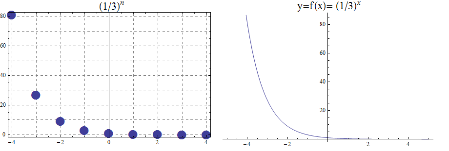
When the base \(b\) is less than 1 the exponential function is decreasing exponentially, as in the case \(f(x) = \left(\frac{1}{3}\right) ^x\).
\begin{array}{llcccccccccl} & x & -5 & -4 & -3 & -2 & -1 & 0 & 1 & 2 & 3 & 4 & 5 \\ & (\frac{1}{3})^x & 243 & 81 & 27 & 9 & 3 & 1 & \frac{1}{3} & \frac{1}{9} & \frac{1}{27} & \frac{1}{81} & \frac{1}{243} \end{array}
17.2.2. Logarithmic Functions
Logarithmic functions are the inverse functions corresponding to exponential functions and are used to solve exponential equations. For example, \(y=2^x\) is solved for \(x\) by inverting \(x=\log_2{y}\). Properties of logarithms follow from this relationship between exponentials and logarithms and properties of the exponentials.
We summarize three important properties of logarithms.
All other properties of logarithmic functions come from properties relating the logarithm as the inverse of the exponential and the equivalence of the logarithm \(a =\log_b m\) with \(b^a=m\).
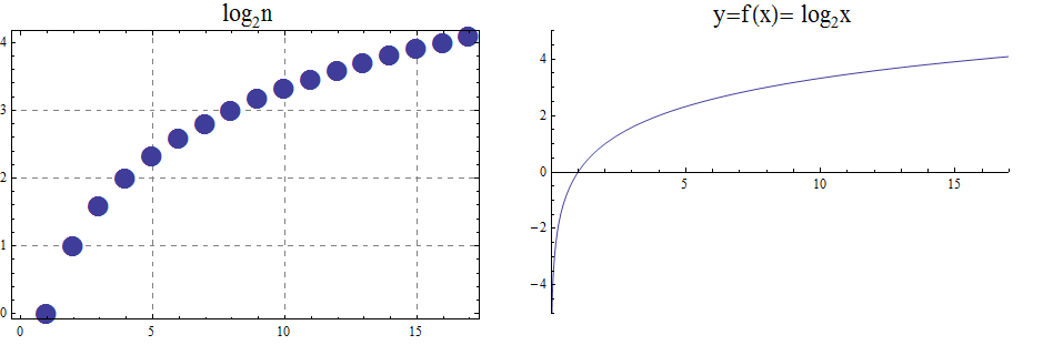
When the base \(b\) is greater than 1, the logarithm function is increasing, as in the case \(f(x) = \log_2 x\).
\begin{array}{llllllcccccc} & x & \frac{1}{32} & \frac{1}{16} & \frac{1}{8} & \frac{1}{4} & \frac{1}{2} & 1 & 2 & 4 & 8 & 16 & 32 \\ & log_2 x & -5 & -4 & -3 & -2 & -1 & 0 & 1 & 2 & 3 & 4 & 5 \end{array}
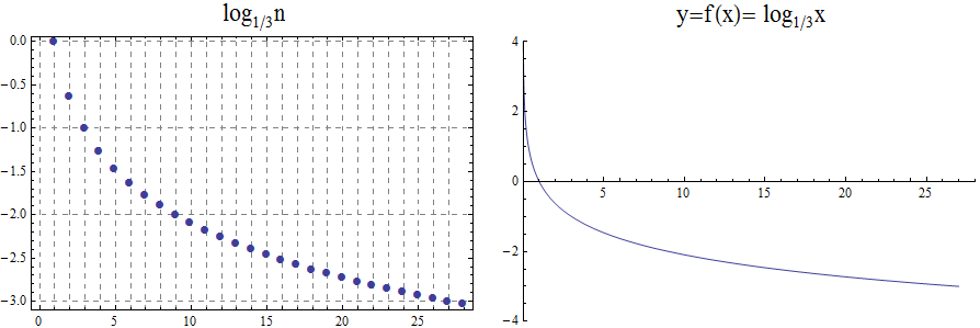
When the base \(b\) is less than 1, the logarithm function is decreasing exponentially, as in the case \(f(x) = \log_{\frac{1}{3}} \ x\).
\begin{array}{llllllcccccl} & x & \frac{1}{243} & \frac{1}{81} & \frac{1}{27} & \frac{1}{9} & \frac{1}{3} & 1 & 3 & 9 & 27 & 81 & 243 \\ & \log_{\frac{1}{3}} x & 5 & 4 & 3 & 2 & 1 & 0 & -1 & -2 & -3 & -4 & -5 \end{array}
17.3. The Floor and Ceiling Functions
The floor and ceiling functions round a real number input to an integer.
-
The floor of x , written as \(\lfloor x \rfloor,\) is the greatest integer that is less than or equal to x . In older textbooks you may see this function named as the greatest integer function and denoted by \([ x ] .\) For example, \(\lfloor -1.5 \rfloor = -2\).
-
The ceiling of x , written as \(\lceil x \rceil,\) is the least integer that is greater than or equal to x . For example, \(\lceil -1.5 \rceil = -1\).
On a number line, the floor of x and the ceiling of x are the consecutive integers such that \(\lfloor x \rfloor \leq x \leq \lceil x \rceil\).
The floor and ceiling functions are step functions: In the plane, their plots look like they are made of horizontal steps.
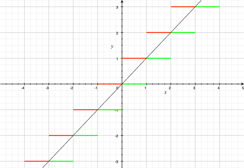
Note that the plot of the floor function, shown in green, is always at the same height or below the graph of the line \(y = x\), and that the plot of the ceiling function, shown in red, is always at the same height or above the graph of the line \(y = x.\)
17.4. Other Functions
MORE TO COME!!