5. Proofs: Basic Techniques
CAUTION - CHAPTER UNDER CONSTRUCTION!
NOTICE: If you are enrolled in the CSC 230 course that I teach at SFSU, you need to use the “CSC230 version” of the book, which I will be updating throughout the semester. The version you are looking at now is the “public version” of the book that will not be updated again before the start of June 2026.
This chapter was last updated on August 18, 2025
Removed statement that universal generalization is used in proofs by mathematical induction.
Contents locked until 11:59 p.m. Pacific Standard Time on May 23, 2025.
Recall from the Logic chapter that an argument is a finite sequence of statements that ends with a final statement, the conclusion, that is based on inferences made from the earlier statements, called premises or hypotheses.
An argument is valid if it is of a form such that if all premises are True then the conclusion must be True, too. An argument is not valid just because it exists! Just as a proposition is a single statement that may be either True or False (but not both), an argument is a finite sequence of statements that may be either valid or invalid (ut not both.)
A proof is a valid argument made up of propositions. In a proof, some premises may be axioms or postulates, which are propositions that we simply ASSUME to be True. Other premises used in a proof may be previously-proven propositions called theorems. There are many other terms used for theorems depending on the context, such as lemma (a minor theorem needed to prove a more important major theorem) and corollary (a theorem that is a conclusion based on a premise that is a more important theorem), but each of these specialized terms describes a theorem.
Key terms and concepts covered in this chapter:
-
Propositional inference rules (concepts of modus ponens and modus tollens)
-
Notions of implication, equivalence, converse, inverse, contrapositive, negation, and contradiction
-
-
The structure of mathematical proofs
-
Proof techniques
-
Direct proofs
-
Proof by counterexample (Disproving by counterexample)
-
Proof by contraposition (proof by contrapositive)
-
Proof by contradiction
-
-
To be added to this chapter after May 23, 2025:
-
logical equivalence and circles of implication
-
5.1. Rules of Inference for Propositions
To create a proof, we must proceed from True propositions to other True propositions without introducing False propositions into the argument. To do this, we use rules of inference, which are ways to draw a True conclusion from one or more premises that are already known to be True (or assumed to be True). That is, a rule of inference is an argument form that corresponds to a tautology, and so is valid.
In the following subsections we will discuss some of the more common rules of inference.
5.1.1. Transitivity Of The Conditional
The following rule of inference is called pure hypothetical syllogism, but we will use the less formal name transitivity. It is the basis of conditional proof in mathematics.
By applying transitivity multiple times, you can build a finite chain of implications of any length you want:
-
\(p \rightarrow p_{1}\)
-
\(p_{1} \rightarrow p_{2}\)
-
\(p_{2} \rightarrow p_{3}\)
-
\(\vdots\)
-
\(p_{k-1} \rightarrow p_{k}\)
-
\(p_{k} \rightarrow r\)
-
\(\therefore p \rightarrow r\)
5.1.2. Rules Of Inference And Fallacies Arising From The Conditional
Recall that if you have propositions \(p\) and \(q,\) you can form the conditional with hypothesis \(p\) and consequent \(q,\) which is written as \(p \rightarrow q\), as well as three other related conditionals.
-
\(p \rightarrow q\), the conditional
-
\(q \rightarrow p\), the converse of \(p \rightarrow q\)
-
\(\neg q \rightarrow \neg p\), the contrapositive of \(p \rightarrow q\)
-
\(\neg p \rightarrow \neg q\), the inverse of \(p \rightarrow q\)
Also, recall that \((p \rightarrow q) \equiv (\neg q \rightarrow \neg p)\). That is, \((p \rightarrow q) \leftrightarrow (\neg q \rightarrow \neg p)\) is a tautology. This means that the conditional is logically equivalent to its contrapositive. The conditional is NOT logically equivalent to either its converse or its inverse, as was shown using truth tables in the Logic chapter.
From the four conditionals you can get two rules of inference and two fallacies. Together, these four argument forms are referred to as the mixed hypothetical syllogisms.
First, here are the two rules of inference.
Next, here are the two fallacies. They are included because they are very common errors to be aware of and to avoid.
The following image uses an Euler diagram of two sets \(A \subseteq B\) to explain why the converse error is a fallacy. The image can also be used to explain why the inverse error is a fallacy.
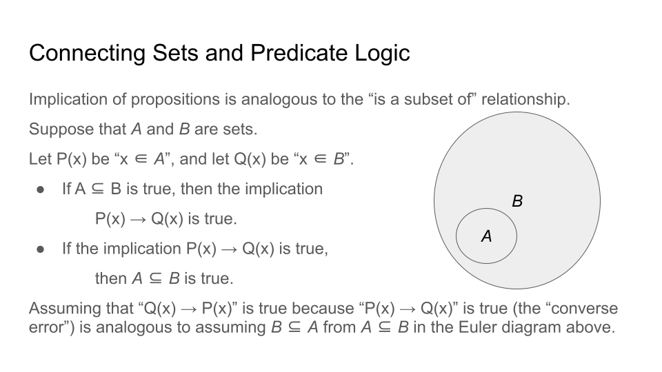
Suppose you were told that \(c\) is an element of \(B\) in the preceding image. Can you determine whether \(c\) is an element of \(A\), too?
5.1.3. Other Common Rules Of Inference
Any tautology of the form \(p \rightarrow q\) can be used to define a rule of inference. In particular, we can define a rule of inference corresponding to the tautology \((p_{1} \land p_{2} \land \ldots \land p_{n})\rightarrow p_{1}\) for each integer \(n \geq 1\). This means that there are at least as many possible tautologies as there are natural numbers! How do we deal with infinitely many tautologies?
In general, there is a small number of rules of inference that are used in most proofs. Proofs often are built up to a large size by applying just a few rules of inference multiple times.
Here are some of the more commonly-used rules of inference. In the remix author’s opinion, it’s better to practice using these rules of inference rather than to focus on memorizing them as formal rules with special names.
There are many more rules of inference we could write down and give names to. Instead, we’ll just list a few tautologies.
5.2. Rules Of Inference for Quantified Statements
In this section, four rules of inference that apply to quantified predicates are presented. In all of these rules of inference, the values of the variable(s) are assumed to be restricted to a universal set \(U.\)
5.2.1. Rules of Inference for Universally-Quantified Predicates
Universal instantiation states that, from the premise that \(\forall x P(x)\) is True, where \(x\) ranges over all elements of the universal set \(U,\) you can conclude that \(P(c)\) must also be True, where \(c \in U\) is any arbitrarily-chosen element of \(U.\)
Universal generalization states that, from the premise that \(P(x)\) is True for every arbitrarily-chosen value of \(x\) that is an element of the universal set \(U,\) you can conclude \(\forall x P(x)\) must also be True, where \(x\) ranges over all elements of the universal set \(U.\)
5.2.2. Rules of Inference for Existentially-Quantified Predicates
Existential instantiation states that, from the premise \(\exists x P(x),\) you can conclude that there must be at least one \(c \in U\) such that \(P(c)\) is true. This allows you to pick a "constant" \(c\) that makes the predicate \(P(x)\) True instead of needing to refer repeatedly to the existential quantifier.
Existential generalization states that, from the premise that \(P(c)\) is True for at least one \(c \in U,\) you can conclude that \(\exists x P(x)\) must also be True.
5.3. Proof Techniques
In this section several examples of formal mathematical proofs are given to illustrate different proof techniques. Many of the techniques correspond to certain rules of inference that were discussed earlier in this chapter.
Each proof starts by stating a conjecture, which is a proposition with undetermined truth value. The goal of each proof is to determine the truth value of the relevant conjecture.
To simplify the description of the proof techniques, we’ll only consider the case where the proof has a single premise \(p\), that is, we’ll always assume that our proof involves a single conditional \(p \rightarrow q\). This may seem like an oversimplification, but it is not: We are simply renaming the conjunction \((p_{1} \land p_{2} \land \ldots \land p_{n})\) of all of the actual premises by using the single propositional variable \(p\), that is we are defining \(p\) by the logical equivalence \(p \equiv (p_{1} \land p_{2} \land \ldots \land p_{n})\)
Here we’ll present examples of proofs using several different techniques. Most of these proofs establish an arithmetic fact that you probably have always known (or assumed) is True; instead, you can focus on the form of the proof: Note the steps that are used, and how the argument flows.
Another important proof technique, mathematical induction, will be discussed in a later chapter.
5.3.1. Direct Proof
In a direct proof, we make an argument that a conditional statement \(p \rightarrow q\) must be True. This means that we can assume that the premise \(p\) is True and apply modus ponens to prove that \(q\) must be True, too.
5.3.2. Proof By Contraposition
In a proof by contraposition, we make an argument that \(p \rightarrow q\) is True by instead first arguing that its contrapositive \(\neg q \rightarrow \neg p\) is True and secondly applying the logical equivalence of the conditional and its contrapositive. Start by assuming that the premise \(\neg q\) is True and apply modus ponens to prove that \(\neq p\) must be True, too, then apply logical equivalence.
5.3.3. Proof By Counterexample
In a proof by counterexample, we disprove a proposition of the form \((\forall x \in D) P(x)\) by arguing that there is at least one value \(c \in D\) such that \(\neg P(c)\) is True.
5.3.4. Proof by Contradiction
In a proof by contradiction, we disprove the proposition \(\neg p\) by making an argument that the conditional \(\neg p \rightarrow (q \land \neg q)\) must be True for some proposition \(q\) and apply the Contradiction Rule to conclude that \(p\) must be True.
Note: Sometimes, we argue instead that the proposition \(((\neg p \rightarrow q) \land (\neg p \rightarrow \neg q))\) must be True, and use the fact that this proposition is logically equivalent to \(\neg p \rightarrow (q \land \neg q)\) and apply the Contradiction Rule.
Here is another example of proof by contradiction.
5.3.5. Proof By Exhaustion (Proof By Cases)
Sometimes it is convenient to break a proof into a finite number of cases. For example, it may be easier to prove a statement that involves an integer by considering a first case where the integer is odd and a separate second case where the integer is even, then combining the two separate cases to create a single proof for all integers \(n.\)
In a general proof by cases, you make an argument that a conditional statement \((p_{1} \lor \cdots \lor p_{n}) \rightarrow r\) must be True. This means that if any one of the "cases" \(p_{i},\) where \(i \in \{ 1, 2, \ldots , n \},\) is True, you can apply the tautology \(p_{i} \rightarrow (p_{1} \lor \cdots \lor p_{n})\) and the transitivity rule of inference to prove that \(r\) must be True, too.
A proof by exhaustion is a special kind of proof by cases where the premise is of the form \((p_{1} \lor \cdots \lor p_{n} \lor \neg (p_{1} \lor \cdots \lor p_{n}) ).\) Notice that this premise must be True since if all of \(p_{1},\) \(p_{2},\)… \(p_{n}\) are False then \(\neg (p_{1} \lor \cdots \lor p_{n})\) is True.
If there are two cases, proof by exhaustion corresponds to using the "proof by cases" rule of inference discussed above in the section "Other Common Rules Of Inference." The tautology can be rewritten in the simpler form \(((p \rightarrow r) \land (\neg p \rightarrow r)) \rightarrow r\) because \(p \lor \neg p\) must always be True.
If there are more than two cases, this corresponds to using the tautology \(((p_{1} \rightarrow r) \land ... \land (p_{n} \rightarrow r) \land (\neg (p_{1} \lor \cdots \lor p_{n}) \rightarrow r)) \rightarrow r\).