1. Introducing Discrete Mathematics
NOTICE: If you are enrolled in the CSC 230 course that I teach at SFSU, you need to use the “CSC230 version” of the book, which I will be updating throughout the semester. The version you are looking at now is the “public version” of the book that will not be updated again before the start of June 2026.
This chapter was last updated on July 9, 2025.
Welcome to the Remix! I hope this textbook provides you an opportunity for a stimulating and intellectually enjoyable learning experience.
Mathematics is one of human civilization’s greatest tools: It involves pattern noticing, collecting, comparing, counting, generalizing, formalizing, and abstracting. The development of mathematics is a continuing work that spans at least 5,000 years and many different peoples and cultures. This development will continue long after you and I are gone - never forget that we are living during an era that will be someone else’s Ancient History!
1.1. What is "Discrete Mathematics"?
There seems to be no universally agreed-upon definition of "discrete mathematics," but I will describe to you my understanding of what the phrase "discrete mathematics" means.
Discrete mathematics is the mathematics people use to study and understand structures that are built from individual objects in a way that the individual objects can still be treated as separate from one another within the structure. In such a structure, the individual objects can be put into categories and counted; it makes sense to ask questions like "What is the next object in the structure after this one?" or "Which other objects are the closest to this one?" (where "closest" could refer to physical distance or could mean most similar in color or size) or "How many objects in the structure have a certain property?" Discrete mathematics is a collection of tools that can be used to answer these kind of questions.
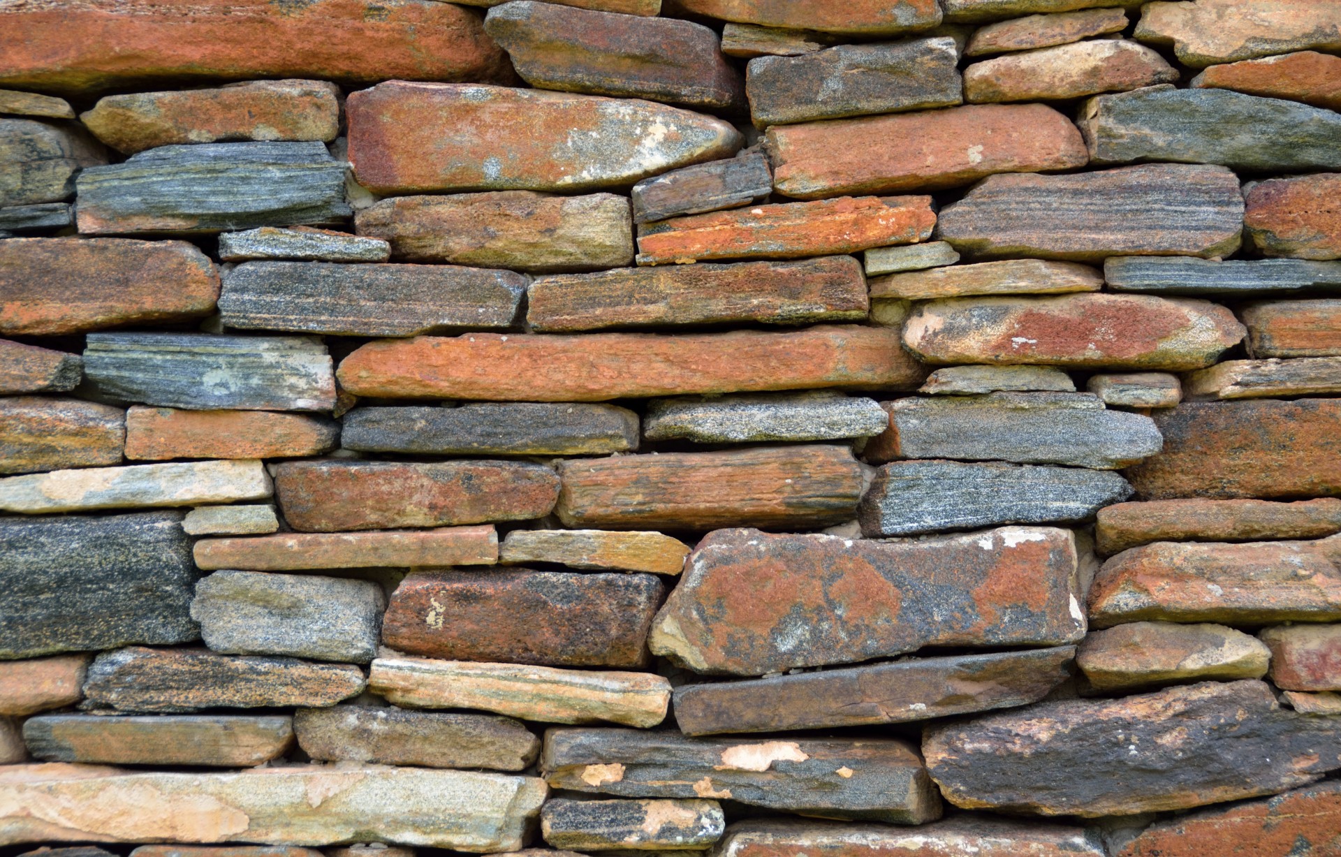
As an example, consider a wall, a structure built from individual stones and bricks, part of which is shown in the image.
The
individual
objects in the structure are
the stones and bricks. You can still identify individual objects even though they were combined to build the larger structure, and can classify
an
individual object
by type (either stone or brick) or by color or by the how close to the top of the wall the object
is. You can try to count the total number of individual objects, and you can count the number of individual objects that are next to any one object you choose. The wall is a (non-mathematical) example of a
discrete structure.
Image credit:
"Vintage Stone And Brick Wall"
by Paul Brennan. The image is dedicated to the public domain under
CC0
.
Here are two more examples of discrete structures.
-
A family of humans can be treated as a discrete structure.
The humans in a family are seen as individuals who can be distinguished from one another. Questions like "Which humans are siblings of this human?" and "Which humans are parents of this human?" and "How many children does this human have?" make sense. -
The set of integers, in the usual order, as represented on a number line is a discrete structure.
It makes sense to ask questions like "What is the next integer after -2?" or "What are the integers that are closest to -2?" for this structure.
Notice that in these examples, the individual objects are of a different nature than the entire structure: Individual bricks and stones aren’t considered a wall, individual humans aren’t considered a family, and individual integers are not a collection of integers.
So what kind of structure is not discrete?

Consider the water in the glass shown in the image. The water in the glass
is
a structure, but for most of human history it has not been seen as made up of objects that are of a different nature than the structure. That is, many generations of humans have recognized the difference between a wall and the individual stones and bricks that make up the wall, but likely have perceived water as being made up of… water. This is why humans tend to use
measurement of quantities
of water, using units such as fluid ounces or milliliters.
In our current era,
we humans understand that the water is built from molecules,
which are of a different nature than the water
"structure,"
but because the molecules are so tiny, numerous, and densely distributed throughout the structure, we humans (except perhaps some scientists and engineers)
still use measurement instead of counting and ignore the individual molecules.
For example, a recipe might call for "8 ounces of water" but never would ask for "7.6 × 10
24
molecules of water." Notice that the measurement units used do not correspond in any natural way to individual molecules or groupings of individual molecules (unless, perhaps, you are a scientist or engineer.)
Also, notice that the glass container itself is another structure in which the individual molecules tend to be ignored.
Image credit:
"Water Glass"
by Peter Griffin. The image is dedicated to the public domain under
CC0
.
Humans use continuous mathematics like calculus to study a structure that is built from objects that are densely distributed throughout the structure. For such a structure, measurement and approximation is more appropriate than counting.
-
The set of real numbers, in the usual order, as represented on a number line is NOT a discrete structure.
It does NOT makes sense to ask about "the next real number after \(\pi\) on the number line" because if we think c is "the next real number after \(\pi\) on the number line" then we can compute the number \(c_{1} = \frac{c+\pi}{2},\) which is the midpoint of the interval with endpoints \(\pi\) and c, so \(c_{1}\) is closer to \(\pi\) than c is, which means \(c_{1}\) is a better candidate for "the next real number after \(\pi\) on the number line" than c … so the concept "the next real number after \(\pi\) on the number line" does not make sense for this structure as such a number cannot exist! We can just keep computing numbers that get closer and closer to \(\pi\) over and over again. Likewise, "the real numbers that are closest to \(\pi\)" do not exist.
Instead, it makes sense to talk about "the real numbers that differ from \(\pi\) by less than \(\epsilon\)" where \(\epsilon\) is some positive real number (The symbol \(\epsilon\) is the Greek letter "epsilon".) By choosing \(\epsilon\) as small as we like, we can describe the real numbers that are as close to \(\pi\) as needed to use as approximations to \(\pi.\) This is why and how limits are defined and used in courses like precalculus and calculus, subjects that involve the real number line.
Note 1: You could use any other real number instead of \(\pi\) in the discussion above because the argument will still be valid. For example, "the next real number after \(-2\) on the number line" and "the real numbers that are closest to \(-2\) on the number line" do not exist since you can choose numbers that get closer and closer to \(-2\) such as \(-1,\) \(-1.5,\) \(-1.75,\) and so on.
Note 2: The technique used to justify that "the next real number after \(\pi\) on the number line" does not exist is called proof by contradiction and will be discussed along with other techniques in the Proofs: Basic Techniques chapter of this textbook.
Note 3: Is \(\pi\) really on the number line? Click here to view an artist’s explanation about where \(\pi\) lies on the number line. Be warned that some of what this artist says (about history, about \(\pi\) being equal to 3.14) is not correct, but the visualization still may be helpful to you.
Note 4: FYI, the set of real numbers is called the continuum in advanced mathematics courses.
1.2. To The Student: Some Things To Know Before You Begin
Here are some things to orient you.
1.2.1. How To Use This textbook
The Remix is designed to build on your previous knowledge, and then build new knowledge and understanding by visiting the topics over and over again. In the next subsection, the basis of foundational mathematical ideas are discussed. You are encouraged to read through all of those foundational topics and to work through the Questions and Challenges.
There are two analogies that I, the remixer, like to use here:
-
Think of the course presented in the Remix as a language course.
You will use this language to talk about mathematics and computer science as you continue along your professional path. You cannot master a new language by learning some words or grammar in the first few weeks of a language course and then "forgetting" that content later, but still succeed in the course and master the language to use beyond the course. You need to assume that everything you learn in this textbook will apply later in the textbook and in your later learning. One of the goals of this textbook is to help you build a broad and rich vocabulary in discrete mathematics and a way of thinking that will apply to your future work. -
Think of the course presented in the Remix as exercising at a gym.
You will build your strength and awareness about your abilities by working out. It may be tempting to watch others "demonstrate" how to do certain exercises and then choose not to do them yourself, but you are selling yourself short. A physical trainer usually knows already what they are capable of doing, so it is no compliment if you tell them "Wow, you’re really strong"… the trainer’s goal is to get you to say "Wow, I’m starting to get really strong!"
1.2.2. Foundations
Learning discrete mathematics requires putting together old ideas in new ways and adding new ideas to your mix.
This subsection highlights some of the ideas you will need to work with in order to get the most out of this textbook. Also, you’ll find opportunities here to practice with the built-in tools that are part of the textbook. Some of these ideas may be old for you, but others will probably be new. To use this textbook effectively, you’ll need to be able to work with each of these ideas with relative ease. If a few of these ideas are brand new to you, that is fine: All of these ideas will be discussed again, much more formally and in greater detail, later in the textbook.
I encourage you to read all of the topics discussed below. Don’t skip anything, even if it looks "old" because there may be some new ways of understanding the old ideas that are introduced and that will be used later in the course.
-
A set is an unordered collection of zero or more objects. You can think of a set as a list of the names of the objects included, but we do not care about the order of the names in the list and we do not care if the list contains duplicate names.
An example is the set of the names of the additive primary colors of light which can be written as \[\{ \text{"red"},\,\text{"green"},\,\text{"blue"},\,\text{"red"} \}\] which contains exactly three elements: "blue", "green", and "red." It does not matter that "red" appears twice, and it does not matter that the order of the colors in the list "blue", "green", and "red" is different from the order used in the previous set notation. We could define the same set with any other list that contains the same three elements, for example, \(\{ \text{"green"},\,\text{"red"},\,\text{"blue"} \}.\)
As you will see in the Set Theory chapter, it is common practice to use uppercase English letters to stand for sets; this is similar to how lowercase letters are used as variables or constants in algebra. For example, you could write \[P = \{ \text{"red"},\,\text{"green"},\,\text{"blue"},\,\text{"red"} \}\] which allows you to refer to the set as P instead of needing to read the list of elements every time you want to talk about the set. This is like using the Greek letter π instead of needing to read off the first few digits of the non-repeating decimal expansion 3.14159265359… every time you refer to that number.-
NOTE 1: In mathematics, a set like \(P,\) that is, \(\{ \text{"red"},\,\text{"green"},\,\text{"blue"},\,\text{"red"} \}\) is treated as a constant, so you cannot remove elements or insert new elements once a set has been defined and described. As an example, if you wanted to insert the name "white" into the set, you would need to define a new set \[ C = \{ \text{"red"},\,\text{"green"},\,\text{"blue"},\,\text{"red"},\,\text{"white"} \}\] that contains four elements by appending "white" to the list used to define the old set P.
-
NOTE 2:
-
One way of creating a new set from two other sets is to form the union of the two sets. The union of two sets is formed by joining the sets.
For example, If \(P = \{ \text{"red"},\,\text{"green"},\,\text{"blue"},\,\text{"red"} \}\) and \(T = \{ \text{"yellow"},\,\text{"red"},\,\text{"blue"} \}\), then the union of the two sets is \(\{ \text{"red"},\,\text{"green"},\,\text{"blue"},\,\text{"red"}, \, \text{"yellow"},\,\text{"red"},\,\text{"blue"} \},\) the set that contains the colors that are in at least one of the sets \(P\) and \(T.\)
-
Another way of creating a new set from two other sets is to form the intersection of the two sets. The intersection is the meeting of the two sets.
For example, If \(P = \{ \text{"red"},\,\text{"green"},\,\text{"blue"},\,\text{"red"} \}\) and \(T = \{ \text{"yellow"},\,\text{"red"},\,\text{"blue"} \}\), then the intersection of the two sets is \(\{ \text{"red"},\,\text{"blue"} \},\) the set that contains the colors that are in both of the sets \(P\) and \(T.\)
Likewise, if \(S = \{ \text{"yellow"},\,\text{"cyan"},\,\text{"magenta"} \},\) the set of additive secondary colors, then the intersection of \(P\) and \(S\) is the set \(\{ \},\) the set that contains zero elements. We call the set \(\{ \}\) the empty set.
-
-
NOTE 3: We can define a subset of any set by selecting zero or more of the members of the set. For example, \(\{ \text{"green"},\,\text{"blue"} \}\) and \(\{ \text{"green"} \}\) are subsets of \(\{ \text{"red"},\,\text{"green"},\,\text{"blue"},\,\text{"red"} \},\) and so is \(\{ \},\) the empty set.
-
NOTE 4: A set can also be defined by a property instead of a list. This will be explained in the Set Theory chapter.
-
-
A one-to-one correspondence between two sets A and B is a pairing of each member of the set A with exactly one member of set B, and each member of set B with exactly one member of set A.
As a first example, the one-to-one correspondence between the set of uppercase English letters and the set of lowercase English letters is represented in the image. You can choose each letter in the upper row and follow the arrow down to the corresponding lowercase letter that it is paired with.
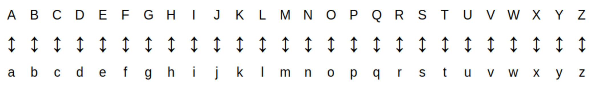
Notice that you could choose any lowercase letter in the image and follow the arrow up to its corresponding uppercase letter. This shows that the one-to-one correspondence
is invertible in the sense that there is a second one-to-one correspondence that can "undo" what the first one-to-one correspondence does.
This is why the arrows in the image point in both directions: It is natural to interpret the arrow as meaning "change case" in either direction.
In fact, the image for the one-to-one correspondence actually represents two
functions
: The first function is the uppercase-to-lowercase conversion that uses only the down arrows, and the second function lowercase-to-uppercase conversion that uses only the up arrows.
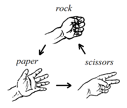
As a second example, consider the game
"rock, paper, scissors."
The image represents the one-to-one correspondence that pairs each element of the set \(\{ \text{"rock"},\,\text{"paper"},\,\text{"scissors"} \}\) with the element of the same set that it loses to.
Image credit: Remixer-created derivative of original work
"THE_GAME_OF_KEN.
(1910)
-
illustration
-_page_315.png"
. According to Japanese Copyright Law (June 1, 2018 grant) the copyright on the original work has expired and is as such public domain. Also, the original work is in the public domain in the United States because it was published (or registered with the U.S. Copyright Office) before January 1, 1930.
_-_illustration_-_page_315.png)
For this one-to-one correspondence, it makes more sense to use arrows that point in only one direction.
In the image, all the arrows point to the winner, so each arrow can be read as "loses to," for example "rock loses to paper".
Note 1: A one-to-one correspondence between a set and itself is called a
permutation.
You will see the term "permutation" again, used with a related but different meaning, in the
Counting: Permutations and Combinations
chapter.
Note 2: "Rock, paper, scissors" is a modern form of a very old game that appears to date back at least 1,800 years to China during the time of the Han dynasty. You can learn more about the history of "rock, paper, scissors" and other intrasitive games at this
Wikipedia link
. The image used in the Remix is derived from one that appears in a
book
published in 1910 that describes the Japanese game stone-
ken
or
jan-ken.
-
A natural number is one of the nonnegative integers . The letter \(\mathbb{N}\) denotes the set of natural numbers, that is, \[\mathbb{N} = \{ 0,\,1,\,2,\,3,\,\ldots \}\] where the three dots are used because we cannot write down the entire list of natural numbers.
-
NOTE: We almost always use the base-ten (decimal) place-value system to represent natural numbers, but later in this textbook you will see that there are other number base systems such as the base-two (binary) place-value system, that are useful in some contexts.
-
WARNING: The definition of natural numbers used in this textbook is an ISO standard, but be aware that other textbooks and sources may use the "nonstandard" definition that the natural numbers are the positive integers. In this textbook, the set of natural numbers ALWAYS include zero as well as the positive integers, which is the standard definition.
-
-
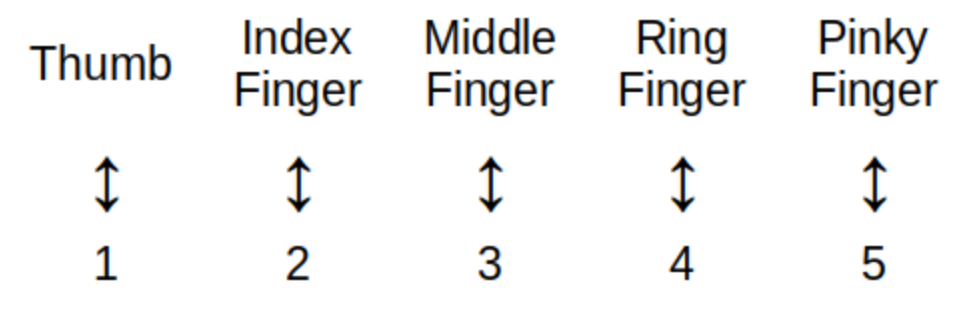
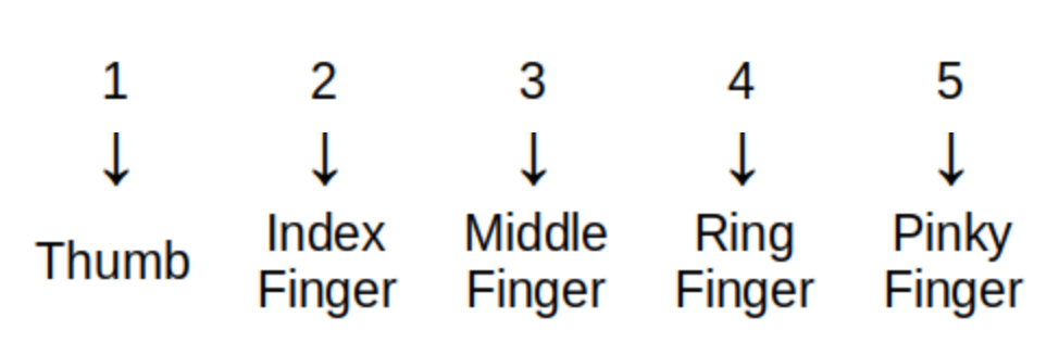
A set is called a finite set if either the set is empty or there is a one-to-one correspondence between the set and \(\{1, 2, \ldots , n \}\) for some positive integer \(n.\) For example, the image represents how a child may "count up to 5" by pairing fingers with the numbers in \(\{1, 2, \ldots , 5 \}.\)
A set that is not a finite set is called an infinite set. Both finite and infinite sets will be discussed in more detail in the Set Theory chapter.
-
You may be surprised to see Counting listed as a topic in a university-level course because you probably learned to count by putting physical objects (like fingers) into a one-to-one correspondence with number words such as "one, two, three, four, five" when you were a young child. That way of counting one by one is fine for small sets, but the counting techniques discussed in this textbook let you count the number of elements in very large finite sets quickly.
The multiplication principle, also called the product rule, is the following statement.
Suppose that we have a procedure that consists of completing two steps, that there are k possible ways to complete the first step, and for each possible way of completing the first step, there are m possible ways to complete the second step. Then there are k⋅m ways to complete the procedure.
As an example, the number of possible strings of 2 characters with the first character being one of the 26 uppercase English letters and second character being one of the 10 Hindu-Arabic numerals is 260 = 26⋅10.
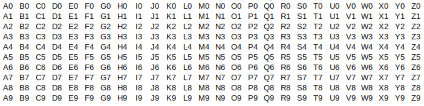
In this case, 26 and 10 are small integers so you can list all possibilities by arranging them in a table as shown in the image. What is important to notice is that this same technique (multiplying k and m ) will work for much larger values of k and m, when creating such a table may be either not helpful or impossible.
Click on "Hint," "Another challenge," and "One last challenge" to reveal the hidden text.
With these additional restrictions, how many different possible passenger vehicle license plate numbers can the state create?
-
The Pigeonhole Principle states that if \(n\) is a positive integer and \(n+1\) objects are going to be assigned to \(n\) categories then one of the categories must be assigned at least 2 of the objects. Click here to see a commonly-used photoshopped image that illustrates this principle.
-
A function from set D to set C is a rule that assigns to each element in D (that is, to each input value) exactly one output value from C. We also say each input value is mapped to the output value. A much more formal definition will be given in the Functions chapter of the textbook, but for now it is enough to understand functions in this way.
-
The rule may be represented by a mathematical equation, a verbal description, a table of paired values, a plot of points, … or even code 😎!
-
The set D of all input values is called the domain of the function.
-
The set C that contains the output values is called the codomain of the function.
-
The range of the function is the set that contains only the output values and no other elements. The range is always a subset of the codomain C, but may not contain every element of C . That is, some elements of C may not be outputs for the function. It is often important to distinguish the range from the codomain; this is discussed in detail in the Functions chapter.
-
Here are some examples of functions with their rules, domains, codomains, and ranges.
-
Any one-to-one correspondence between two sets A and B can be viewed as a function \(f\) from A to B .
-
The rule for \(f\) is given by the pairing of elements in A with elements in B.
-
The domain of \(f\) is the set A.
-
The codomain of \(f\) is the set B.
-
The range of \(f\) is the set B, too, because every element in B is paired with an element in A by the one-to-one correspondence.
Notice that the one-to-one correspondence can be used to define another function g from B to A with domain B, codomain A, range A, and rule given by the pairing of elements in B with elements in A. The two functions \(f\) and g are called inverse functions because \(f\) and g "invert" or "undo" each other. Inverse functions will be discussed in more detail in the Functions chapter.
-
-
The floor of x , \(\lfloor x \rfloor,\) and the ceiling of x , \(\lceil x \rceil,\) are two functions defined for all real numbers as follows:
-
\(\lfloor x \rfloor\) is the greatest integer less than or equal to x. For example, \(\lfloor -1.5 \rfloor = -2\) and \(\lfloor 6.3 \rfloor = 6\)
-
\(\lceil x \rceil\) is the least integer less than or equal to x. For example, \(\lceil -1.5 \rceil = -1\) and \(\lceil 6.3 \rceil = 7\)
-
The domain of both the floor and ceiling functions is the set of all real numbers, \(\mathbb{R}.\)
-
The range of both the floor and ceiling functions is the set of all integers, \(\mathbb{Z}\) (NOTE: The German word for "numbers" is Zahlen, which is why the letter \(\mathbb{Z}\) is used for the integers.)
-
The codomain of these two functions can be chosen depending on the context. If we only need to consider output values we could choose the codomain to be the same set as the range, \(\mathbb{Z},\) but if we want to plot these two functions in the xy coordinate plane we would choose the codomain to be the set of real numbers, \(\mathbb{R}.\) This is discussed in the Functions chapter.
The floor and ceiling functions are discussed in more detail in Appendix: Library of Functions.
-
-
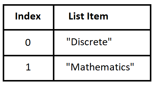
In Python, a list can be used to represent a function with inputs the valid integer indices for the list and outputs the values stored in the list. In an earlier example, we defined list L to be ["Discrete", "Mathematics"] and then evaluated L[0] and L[1] to access the strings stored in the list.
Note for programmers: In reality, the items in the list are references to objects that implement the two strings. That is, the list items are neither the strings nor the objects that implement strings but references to those objects, which are located elsewhere in memory. -
The rule "Return the first character of the input Unicode string."
-
The domain is the set of all strings of length greater than or equal to 1 that contain Unicode characters.
-
The range is the set of all Unicode characters.
-
We would need to decide what the codomain should be in this context: It could be the same as the range, or we could use the larger set of all strings that contain Unicode characters (including the empty string "".)
-
-
\(f(x) = x^{2}\) from the set of real numbers to the set of real numbers.
-
The domain and codomain are both the set of real numbers.
-
The range is the set of nonnegative real numbers.
-
-
\(g(x,\,y) = xy + y\) where x and y are real numbers.
-
The domain is the set of ordered pairs of real numbers.
-
The range is the set of all real numbers. The codomain is the same as the range.
-
-
See the Appendix: Library of Functions for other functions you should be familiar with.
Here is another example.
-
A sequence is a function from the natural numbers, or a subset of the natural numbers, into another set (e.g., the natural numbers, or the real numbers, or a nonnumerical set.) For example, we can define a sequence by the rule \[a_{i} = 2i+1 \text{ for every natural number } i \] which describes the sequence of positive odd integers \(a_{0} = 1,\) \(a_{1} = 3,\) \(a_{2} = 5,\) and so on.
-
NOTE 1: It is common to use i as a variable in sequence notation because i is the initial letter of the word index. This i has nothing to do with the complex number \(\sqrt{-1}.\) Mathematicians recycle and reuse letters!
-
NOTE 2: It is traditional to write the input variable for a sequence as a subscript instead of putting it between parentheses. In the preceding example, \(a_{i} = 2i+1\) has the same meaning as \(a(i) = 2i+1\).
-
NOTE 3: The output values of a sequence are called terms. For example, the 0th term of the sequence is \(a_{0} = 1,\) the 1st term of the sequence is \(a_{1} = 3,\) and so on.
-
-
A finite sequence is a sequence that is defined for only a finite subset of \(\mathbb{N}.\) That is, the set of input \(i\) values that make sense for the sequence is a finite set.
For example, a child counting up to five on the fingers of one hand is defining the sequence called \(\textit{fingers}_{i}\) that is represented by the image.
Technically, the sequence \(\textit{fingers}_{i}\) shown in the image is the inverse of the child’s actual counting sequence. Because the child assigns to each finger "input" exactly one number "output," the arrows would point up from a finger to the corresponding number.
The sequence \(\textit{fingers}_{i}\) can be written, formally, as \begin{equation} \begin{aligned} \textit{fingers}_{1} {} & = \text{"Thumb"} \\ \textit{fingers}_{2} {} & = \text{"Index Finger"} \\ \textit{fingers}_{3} {} & = \text{"Middle Finger"} \\ \textit{fingers}_{4} {} & = \text{"Ring Finger"} \\ \textit{fingers}_{5} {} & = \text{"Pinky Finger"} \\ \end{aligned} \end{equation} but it is much more common to list the terms of the sequence in order: "Thumb," "Index Finger," "Middle Finger," "Ring Finger," "Pinky Finger."
Notice that Java arrays and Python lists are implementations of the mathematical concept of a finite sequence where the domain is the set of \(i\) values \(\{0, 1, \ldots , n \}\) for some natural number \(n.\)
An infinite sequence is a sequence that is not a finite sequence, that is, the there are infinitely many \(i\) values that make sense as inputs for the sequence. For example the sequence \[ \text{isOdd}_{i} = \begin{cases} \text{1} & \text{ if } i \text{ is odd} \\ \text{0} & \text{ if } i \text{ is even} \\ \end{cases} \] is an infinite sequence with domain the integers that has only two output values.
-
A bitstring is a finite sequence of the bits 0 and 1. Bitstrings are written as a string of 0s and 1s without spaces or commas between the terms of the sequence; for example, 01101011 is a bitstring of length 8. Bitstrings can be used to represent a sequence of answers to "Yes-No" or "True-False" questions, with "1" representing "Yes" or "True" and "0" representing "No" or "False." Bitstrings can also be used to represent numbers in binary notation, which will be discussed in the Number Bases chapter.
-
Summation notation is a "shortcut" used to abbreviate a sum of a finite sequence of numbers, called addends, when the sequence contains a large number of addends.
As an example, the sum \(1+3+5+7+9+11+13+15+17+19\) is abbreviated as \(\sum\limits_{i=0}^{9}(2i+1)\).
As another example, the sum of the first \(500\) positive odd integers, \(1+3+5+\ldots+995+997+999\), is abbreviated as \(\sum\limits_{i=0}^{499}(2i+1)\).-
NOTE 1: The variable i used in summation notation is called the index of summation and the symbol \(\sum\) is the capital Greek letter "sigma." To compute the value of the sum, you generate the sequence of addends by substituting each integer value, starting with the lower limit written below the sigma and stopping at the upper limit written above the sigma, for i into the algebraic expression or function written to the right of sigma, then find the sum of all the numbers in the sequence.
-
NOTE 2: "Infinite sums," more properly called infinite series, are not discussed in the Remix. The sum of an infinite series is defined as the limit of its sequence of partial (finite) sums, and "limits" is a topic from continuous mathematics, not discrete mathematics.
Another use of infinite sum notation is to represent the generating function of a sequence, which is discussed in some discrete mathematics textbooks but not in the Remix. If you want to learn about generating functions, you can read about them in Oscar Levin’s Discrete Mathematics: An Open Introduction, 4th edition .
-
-
Recursion is a process that defines an object, or computes a value, or describes the construction of an object or set of objects, using steps that refer to one or more previously completed steps.
-
Recurrence relations consist of one or more equations that define a sequence or a function with domain \(\mathbb{N}.\)
-
In English, there are four types of sentences, depending on what is being communicated: statements (or declarative sentences), commands, exclamations, and questions. A proposition is a statement that declares a fact that is either True or False (but not both!) In mathematics, we are usually most interested in analyzing and verifying propositions.
-
A predicate is an incomplete proposition that contains one or more variables that need to be filled in to complete the proposition. One example of a predicate is "My major is \(\rule{12mm}{.5pt}\)." Notice that this becomes a proposition once the blank, which represents the variable in this case, has been filled in.
Another example of a predicate is "The positive integers m and n are prime numbers." Again, this becomes a proposition once values are substituted for the two variables.
In this textbook, predicates will often be written in a way similar to functions: + \[ P(m, n) : \text{"The positive integers } m \text{ and } n \text{ are prime numbers."} \] Notice that the output of the predicate is a statement but the output does not tell us whether the statement is True or False - think of this like a programmer: The return value is a string, not a Boolean.
Two predicates are equivalent if for every possible substitution for the variables, the statement produced by the first predicate is true if and only if the statement produced by the second predicate is true.
-
An algorithm is a finite sequence of commands and statements that describe a process for completing a task.
It’s likely that you have learned how to perform many algorithms in your previous mathematics education, but in this textbook (and in computer science in general) it is more important that you learn how to analyze and compare algorithms.
One example is the following (correct but inefficient) algorithm for division of positive integers.-
Task: Given two positive integers a and b, compute the quotient q and remainder r so that
\(a = q \cdot b + r\) and \(0 \leq r < b.\) -
Input: Two positive integers a and b
-
Steps:
-
Set r equal to a and set q equal to 0.
-
If r is greater than or equal to b
-
set r equal to r - b
-
add 1 to q
-
-
If r is greater than or equal to b then repeat step 2
-
-
Output: Integers q and r such that both \(a = q \cdot b + r\) and \(0 \leq r < b.\)
-
q is the quotient, that is, the number of times each of the two assignments under step 2 was executed.
-
r is the remainder, that is, the result of the last execution of step 2, so \(r = a - q \cdot b.\)
-
-
-
Based on the case \(b=2\) in the division algorithm discussed above (and the Challenge), every integer a can be written in the form \(a = q \cdot 2 + r\) where q is an integer and \(0 \leq r < 2.\) The integer a is even if \(r=0\) and is odd if \(r=1.\) So we have a precise formal way of understanding and discussing odd and even integers - this may seem unnecessary (or even completely silly), but as you continue reading this textbook you will see that precise formal definitions and descriptions are useful when you need either to justify that certain statements are true or to validate that certain processes always produce correct and expected results.
-
Suppose that \(a\) and \(b\) are integers, which could be positive or negative or zero. The integer b is called a factor of a (or divisor of a ), and a is called a multiple of b if \(a = q \cdot b\) for some integer q. For example, 2 is a factor of 10, and 10 is a multiple of 2, because \(10 = 5 \cdot 2.\) As another example, \(-2\) is a factor of 10, and 10 is a multiple of \(-2\) because \(10 = (-5) \cdot (-2).\)
-
A positive integer n that is greater than 1 is called prime if the only positive integer factors of n are 1 and n itself, and is called composite otherwise. For example, 2 is prime since its set of positive integer factors is \(\{ 1,\,2 \}\), but 6 is composite since its set of positive integer factors is \(\{ 1,\,2,\,3,\,6 \}\).
-
NOTE: The integer 1 is considered neither prime nor composite. The reason for this is beyond the scope of this textbook but would be discussed in a more advanced math course in ring theory .
-
-
Two integers a and b are called relatively prime if the only common positive integer factor of a and b is 1; this is equaivalent to stating that the two integers do not share any prime factors. For example, 10 and 21 are relatively prime integers.
-
A relation on the sets A and B is an association between elements from set A and set B ; A and B are often the same set. Relations will be defined much more formally and precisely in the Relations chapter of the textbook.
Here are some examples of relations:-
The ordering relation "is less than," \(x < y,\) for real numbers x and y. So \(3 < 4\) but \(5 \nless 4.\) The slash through the "<" symbol means that "5 is not related to 4" in the way we want.
The orderings \(>\), \(\geq\), and \(\leq\) are also examples of relations. -
The equality relation \(s=t\) for any elements s and t of the same set A.
A related example is inequality, \(s \neq t.\) -
The divisibility relation "a is a divisor of b" (or " a divides b ") for integers a and b; this is sometimes written as \(a \mid b.\) So for example, \(2 \mid 4\) but \(3 \nmid 4.\)
-
For two integers a and b, we say that "a has the same parity as b" if either both a and b are odd or both a and b are even.
-
Any function \(f\) with domain A and codomain B is a relation since the function associates each element a in A with exactly one element b of B , namely \(b = f(a)\).
-
A relation can also involve more than two sets. As an example, imagine a database of records that has three fields: a student’s name, a student’s college identification number, and the student’s major. The database can be viewed as a set R of ordered triples. So, for example, if a student named Chris Garcia has identification number 900123001 and is a Computer Science major, the set R would contain as an element the ordered triple ("Chris Garcia", 900123001, "Computer Science").
-
-
A graph is a mathematical object that consists of vertices (also called nodes ) that are connected by edges. Graphs are often represented by drawings like the ones shown in the following examples, but you can also represent a graph in other ways that are easier and more efficient to use in code; this will be discussed in the Graphs chapter.
The drawing of a graph is not treated like a geometric polygon: The only two points "on an edge" are the edge’s endpoints. Edges are just connectors between vertices and points that are not indicated as endpoints of an edge are ignored. Also, in a drawing of a graph, the lengths of edges and the straightness or curvedness of edges are not important, just the connections between the edges' endpoints.
| Some high school-level textbooks use the term vertex-edge graph to distinguish this type of graph from graphs (that is, plots of points in the \(xy\)-plane) for equations, functions, or statistical data. |
Keep in mind that a graph is NOT the same as a drawing of the graph. In fact, a graph can usually be drawn in many different ways that may look very different. What is important is the connections, represented by the edges, between pairs of vertices.
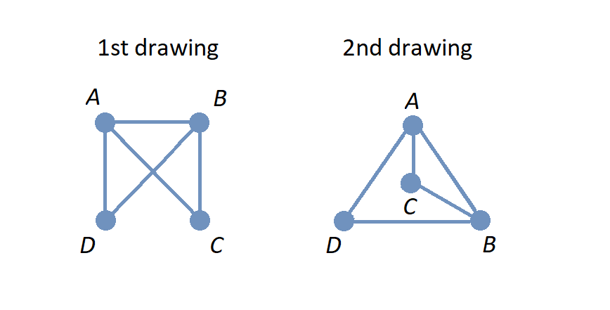
In the image, two different drawings are shown for the same graph. Notice that in each drawing, the connections between pairs of vertices are the same: The only pair of vertices that is not connected by an edge is \(\{ C, D \}.\)
Also notice that there is no vertex drawn where the two edges cross in the 1st drawing on the left, so this graph has 4 exactly vertices: \(A,\) \(B,\) \(C,\) and \(D.\)
A graph can represent relationships between pairs of people.
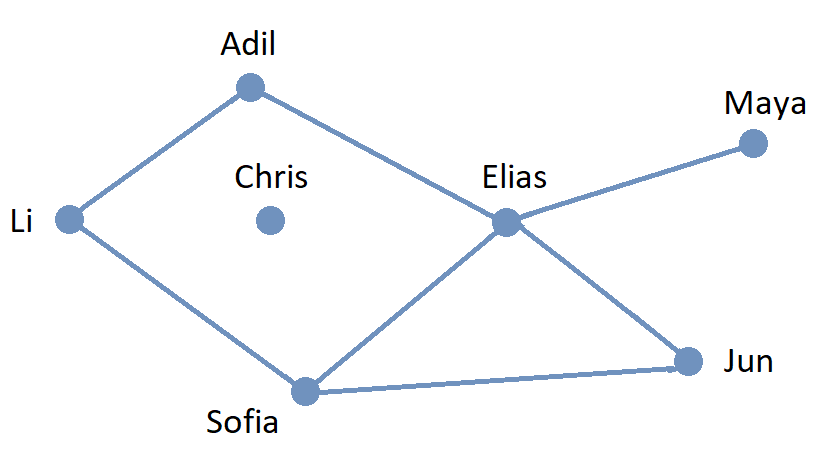
Here is a graph that represents whether pairs of students are enrolled in at least one class together. Each of the 7 vertices represents a student, and each of the 7 edges represents a pair of students who are enrolled in a class together.
The graph indicates that Adil and Elias are enrolled in at least one class together and that Elias and Maya are enrolled in at least one class together.
Here are some other examples of graphs.
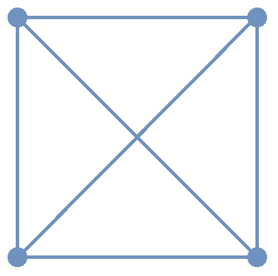
A complete graph is a graph in which every pair of distinct vertices are the endpoints of exactly one edge. The image shows the complete graph on 4 vertices. Notice that two edges appear to "intersect" but there is no vertex drawn where the edges cross, so these edges do not have any points in common - as stated above, an edge contains only its endpoints.
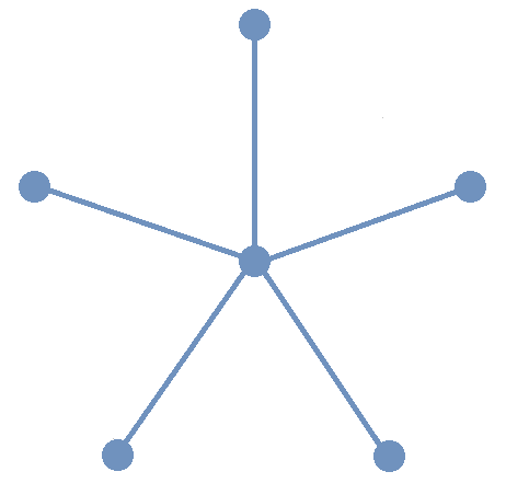
A star graph is a graph that has one central vertex that is one of the endpoints of every edge in the graph. The image shows the star graph on 6 vertices. The star graph is one example of a tree, a graph in which for every pair of distinct vertices there is exactly one path of edges that can be used to connect the vertices. Some of the many applications of trees in computer science will be discussed in the Trees chapter.
The design of this book is to introduce each concept informally, as was done for the preceding foundational ideas, then notice properties and patterns, generalize from what has been noticed, and formalize the ideas to prepare for even deeper analysis.
And congratulations if you read through all of those foundational mathematical ideas in this subsection and worked through all the Questions and Challenges! If you compare the list of ideas to the Table of Contents, you will see that you have touched on every one of the topics that will be discussed in this textbook!
1.2.3. On-Demand Math Resources and Library Of Functions Appendices
Two appendices to this textbook contain additional mathematics that you may need to review as you work your way through the textbook.
1.2.4. Do I Need To Know How To Program In Python?
You are NOT expected to know the Python programming language before you start this course.
As you’ve seen above, this textbook contains Python code snippets that are designed to aid your understanding of the mathematical concepts. It is NOT one of the goals of this textbook to teach you Python, but instead "just enough Python" to be able to examine, run, and alter the existing code snippets.
The appendices "An Introduction to Python" and "Python Syntax Examples" cover most of the basic concepts you will need from the Python programming language.
1.3. Applications of Discrete Mathematics
Remixer’s Note: This section is taken from the original “Discrete Math” book, with only a few minor edits.
Discrete mathematics is applied in many areas including the physical, engineering, and increasingly, the social sciences.
1.3.1. Applications to Applied Mathematics
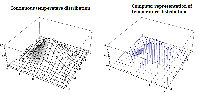
Most problems that involve computational methods, need to be solved using computers. Rather than solve for the temperature map of an entire planar region, we solve for the temperature using a discrete set of mesh or grid of points on a representative subset of the planar region.
1.3.2. Applications to Information Technology and Computer Science
Discrete mathematics is needed for computer science as information and data is stored digitally. Digitally represented data is inherently discrete and is processed using discrete methods. For example a course grid discrete representation of the 2-d temperature distribution from the plate above could be:
\( \left(\begin{matrix}1&1&1\\2&4&8\\3&9&27\\4&16&64\\5&25&125\\\end{matrix}\right) \)
A voter registry may have voters in a database accessible from a list:
\( \left(\begin{matrix}John\ Smith\\Raheem\ Johnson\\.\\.\\.\\Sarah\ Muller\\\end{matrix}\right) \)
Which may need to be accessed and sorted, say geographically or alphabetically.
1.3.3. Applications to Data Science
Data science solutions to many problems use machine learning algorithms that are inherently discrete in nature. The information that needs processing is discrete, as are the basic problems in data science such as classification or clustering problems. In particular
-
Information consisting of data sets is represented using various data structures including graphical structures such as trees. Data science methods and algorithms involve procedures that manipulate these graphical structures to, for example, networks, classification trees, and decision trees.
-
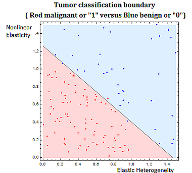
Classification problems are discrete in nature. Classifying tumors as malignant or as benign involves trying to predict if a variable \(Y\) that we can think of as taking on two values either \(0\) or \(1\) either malignant or benign. There are various algorithms used in classification problems, such as the binary tumor classification, including methods from probability.
1.3.4. Applications to Engineering
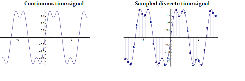
Digital signal processing involves taking a video, audio, or other signal like temperature, pressure, position and velocity, which is continuous, digitizing it and then processing the digital signal mathematically.
1.3.5. Applications of Combinatorics
Combinatorics involves in part the study of counting the number of objects, satisfying a specified condition, from sets of variable size. Enumeration and combinatorics is important in many areas and examples including:
-
Calculating the number of steps an algorithm needs to process a data set of variable size \(𝑛\). This problem is called the computational cost of the algorithm as a function of \(𝑛\).
-
Calculating the possible number of codes in a cryptographic code system
1.3.6. Applications of Graph Theory
Graph theory , which is the study of structures constructed with nodes and the edges joining them, has applications in many fields including,
-
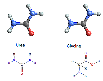
Chemistry - representing molecular bonding and structure
-
Information technology and computer science - ranking pages on the internet, with pages considered as nodes and page links as edges.
-
Industrial engineering and network optimization
-
Traffic routes (computer, internet, air, highway, subway systems) can be represented with stations as nodes and connections as edges.
-
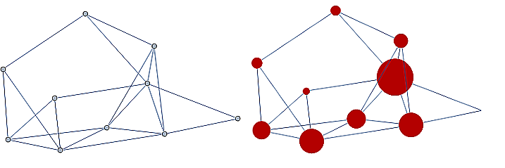
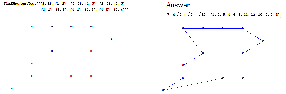
Often we are interested in finding an optimal path in a network such as in the following example, finding the shortest tour over a series of towns on a map.
-
An example of the shortest tour problem, is shown below, using a software solution.
1.3.7. Applications of Probability and Statistics
Many probability assignments are based on counting and combinatorial methods.
-
If we assume that the likelihood of rain is the same on any day in the month of September, we might be interested in the probability that it rains on \(0\) days, it rains on exactly \(1\) day, exactly \(2\) days, etc. Such probability assignments are called discrete distributions, by contrast with continuous distributions like the bell curve.
-
Also probability and statistical techniques are often used in data science. The binary classification problem, of say classifying a tumor as malignant or benign, uses a statistical modeling technique, called regression, specifically logistic regression to determine the strength of the relationship between the independent variable, and dependent heterogeneity variable. In the tumor grading example the independent variable would be \((x_1,x_2 )\) (elastic heterogeneity, nonlinear elasticity), and the dependent variable would be \(Y\), classified as \(0\), or \(1\), (malignant or benign).
1.3.8. Applications to Social Sciences
Discrete mathematical techniques are important in understanding and analyzing social networks including social media networks.
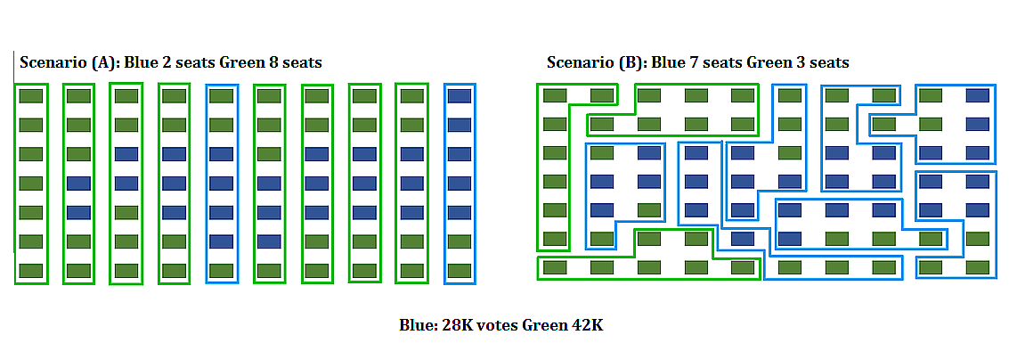
The mathematics of voting is a thriving area of study, including mathematically analyzing the gerrymandering of congressional districts to favor and/or disfavor competing political parties. The following example illustrates some of the fundamental ideas related to gerrymandering.
Consider a fictitious state made up of \(10\) congressional districts with \(7\) thousand voters in each district. To win a district a party (Green or Blue) needs to win \(4\) thousand or more votes. Consider the following two districting map scenarios. In each scenario, the blue party earns \(28\) thousand votes, and the green party earns \(42\) thousand votes. In scenario \(A\), the blue party wins \(2\) out of \(10\) districts, but in scenario \(B\) it wins \(7\) out of \(10\) districts.
1.4. Links to the Informal Definitions in this Chapter
For your reference in the future, here are direct links to most of the bullet points in the list of foundational ideas discussed in this section.
Sets , including subsets, the empty set, unions of sets, and intersections of sets
One-to-one correspondence , including the example "rock, paper, scissors"
Counting , including the Multiplication Principle and Pigeonhole Principle
Functions , including domain, codomain, range, inverse function, and the floor and ceiling functions \(\lfloor x \rfloor\) and \(\lceil x \rceil\)
Sequences , including index and terms
Recurrence Relations , including closed forms
Algorithms , including the Division Algorithm