7. Sequences and Recursion

CAUTION - CHAPTER UNDER CONSTRUCTION!

This chapter was last updated on March 3, 2025.
Contents locked until 11:59 p.m. Pacific Standard Time on May 23, 2025.

Sequences are functions with domain a nonempty subset of the natural numbers. That is, sequences are ordered lists of objects indexed by some or all of the natural numbers. The indexed objects in the list are called the terms of the sequence and may be any kind of object - numbers, sets, functions, strings, steps of a proof, steps of an algorithm, etc.

Recursion is a process that you can use to define an object, compute a value, or describe the construction of an object or set of objects, by using a sequence of steps where each step after the initial step refers to one or more previously completed steps.

Key terms and concepts covered in this chapter:

  • Sequences

  • Recursive mathematical definitions

    • Recursive definitions of sequences and functions

      • Factorials

      • Arithmetic and geometric progressions

      • The Fibonacci sequence (also called the Fibonacci numbers)

      • Other sequences and functions

    • Recursive definitions of sets of objects (e.g., rooted trees, valid Java identifiers)

    • The "Towers of Hanoi" game

  • Recurrence relations

    • Solving recurrence relations

7.1. Sequences

A sequence is a function \(s\) from a nonempty subset of the natural numbers \(\mathbb{N} = \{ 0, 1, 2, 3 \ldots \}\) to a set \(C.\) That is, the domain of the sequence is some set of nonnegative integers, and the codomain can be any set. Each "input" value of \(n\) in the domain is called an index. The "outputs" of the sequence are called the terms of the sequence, and are usually denoted by \(s_{n},\) which is usually used instead of the function notation \(s(n),\) but the meaning is the same: The output value that corresponds to the input \(n.\)

7.1.1. Sequences of Numbers

Two common ways to describe or define a sequence of numbers are

  • a single formula, called a closed form for the sequence, that can be used to compute a term from the value of the index \(n,\) or

  • a recursive rule that includes

    • stating the values of the first few terms of the sequence, called the initial value(s) of the sequence, and

    • a recurrence relation that describes how the \(n\)th term of the sequence \(a_{n}\) can be computed using one or more terms that have index less than \(n.\)

In this subsection, several examples of sequences of numbers are presented. You may have seen some of these sequences in your previous mathematics experience but others may be new to you.

An arithmetic sequence is a sequence of numbers generated by a linear expression.

Example 1 - Arithmetic Sequences

Consider the sequence \(a_n=3n+1\) defined for all natural numbers \(n.\) The first 5 terms of this sequence are shown below.

\(a_0=\ 3\left(0\right)+1=1\)

\(a_1=\ 3\left(1\right)+1=4\)

\(a_2=3\left(2\right)+1=7\)

\(a_3=3\left(3\right)+1=10\)

\(a_4=3\left(4\right)+1=13\)

Notice that this sequence can be defined recursively using a recurrence relation : \[a_0=1 \text{ and } a_n=a_{n-1}+3 \text{ for } n \in \mathbb{N}_{>0}.\] So

\(a_0=1\)

\(a_1=a_{1-1}+3=a_0+3=1+3=4\)

\(a_2=a_{2-1}+3=a_1+3=4+3=7\)

\(a_3=a_{3-1}+3=a_2+3=7+3=10\)

\(a_4=a_{4-1}+3=a_3+3=10+3=13\)

Notice that an arithmetic sequence is determined by an initial term and a common difference. The arithmetic sequence \(a_n=3n+1\) is the sequence with initial term \(a_0=1\) and common difference \(d=3\). The general arithmetic sequence is \(a_n=c + d\cdot n\) with initial term \(c\) and common difference \(d.\)

A geometric sequence is a sequence of numbers generated by an exponential expression.

Example 2 - Geometric Sequences

Consider the sequence \(b_n=2\cdot\ 3^n\) defined for all natural numbers \(n.\) The first 5 terms of this sequence are shown below.

\(b_0=2\cdot\ 3^0=2\)

\(b_1=2\cdot\ 3^1=6\)

\(b_2=2\cdot\ 3^2=18\)

\(b_3=2\cdot\ 3^3=54\)

\(b_4=2\cdot\ 3^4=162\)

Notice that this sequence can be defined recursively using a recurrence relation : \[b_0=2 \text{ and } b_n=3\cdot b_{n-1} \text{ for } n \in \mathbb{N}_{>0}.\] So

\(b_0=2\)

\(b_1=3\cdot b_{1-1}=3\cdot2=6\)

\(b_2=3\cdot b_{2-1}=3\cdot6=18\)

\(b_3=3\cdot b_{3-1}=3\cdot18=54\)

\(b_4=3\cdot b_{3-1}=3\cdot54=162\)

Notice that a geometric sequence is determined by an initial term and a common ratio. The geometric sequence \(b_n=2\cdot\ 3^n\) is the sequence with initial term \(b_0=2\) and common ratio \(r=3\). The general geometric sequence is \(b_n=c \cdot r^n\) with initial term \(c\) and common ratio \(r.\)

The factorial is usually defined using a recurrence relation, but with its own notation that does not use a subscript for the index.

Example 3 - The Factorial Function

The factorial of a natural number can be treated as a term of a sequence, called the factorial function. The commonly-used notation for a term of this sequence is \(n!\) and the sequence is defined as \[n! = n \cdot (n-1) \cdots 2 \cdot 1\] with \(1! = 1\) and \(0! = 1.\)

Notice that the factorial can be defined a bit more precisely by using the recurrence relation \[0!=1 \text{ and } n!=n\cdot (n-1)! \text{ for } n \in \mathbb{N}_{>0}.\] So the first few values of the factorial are

\(0!=1\)

\(1!=1\cdot (1-1)!=1\cdot1=1\)

\(2!=2\cdot (2-1)!=2\cdot1=2\)

\(3!=3\cdot (3-1)!=3\cdot2=6\)

\(4!=4\cdot (4-1)!=4\cdot6=24\)

The next sequence is the very famous Fibonacci numbers, named for the Italian mathematician Fibonacci who was also known as Leonardo of Pisa. However, this sequence and its properties were known and discussed by Indian poets and mathematicians such as Pingala, Virahanka, and Hemachandra before Fibonacci was born. The sequence became known to Europeans when Fibonacci used the sequence in his 1202 book Liber Abaci to solve a counting problem that involves breeding pairs of rabbits
The book Liber Abaci ("Book of Calculation") is credited with popularizing the use of the base-ten Hindu-Arabic numeral system in Europe, too.

Example 4 - The Fibonacci Numbers

The Fibonacci sequence can be defined recursively as \[f_{0}=0, \, f_{1}=1, \text{ and } f_{n} = f_{n-1} + f_{n-2} \text{ for } n \geq 2.\]

\(f_{2} = f_{2-1} + f_{2-2} = f_{1} + f_{0} = 1+0 = 1\)

\(f_{3} = f_{3-1} + f_{3-2} = f_{2} + f_{1} = 1+1 = 2\)

\(f_{4} = f_{4-1} + f_{4-2} = f_{3} + f_{2} = 2+1 = 3\)

\(f_{5} = f_{5-1} + f_{5-2} = f_{4} + f_{3} = 3+2 = 5\)

\(f_{6} = f_{6-1} + f_{6-2} = f_{5} + f_{4} = 5+3 = 8\)

\(f_{7} = f_{7-1} + f_{7-2} = f_{6} + f_{5} = 8+5 = 13\)

Note: The definition used in this textbook matches the ones used in several textbooks, but be warned that other may use definitions that are slightly different (e.g., some sources state the initial values as \(f_{0}=1\) and \(f_{1}=1.\)

7.1.2. Non-numerical Sequences

As mentioned above, the terms of a sequence can be any object. Here are some examples.

Example 5 - A sequence of functions

Consider the sequence \(p_{n}(x)\) of functions that are defined for real number inputs \(x.\)

\(p_{0}(x) = 1,\) that is, the constant function 1,

\(p_{1}(x) = x,\)

\(p_{2}(x) = x^{2},\)

\(p_{3}(x) = x^{3},\)

and in general,

\(p_{n}(x) = x^{n}.\)

This is the sequence of \(n\)th power functions. The subscript of each of the functions matches the power that the input, \(x,\) will be raised to.

Notice that we can define the sequence recursively by \[p_{0}(x)=1, \, f_{1}=1, \text{ and } p_{n}(x) = x \cdot p_{n-1}(x) \text{ for } n \geq 1.\]

The ordered list of steps used in an algorithm is a sequence.

Example 6 - An algorithm for long division
  • Task: Given two positive integers a and b, compute the quotient q and remainder r so that
    \(a = q \cdot b + r\) and \(0 \leq r < b.\)

  • Input: Two positive integers a and b

  • Steps:

    1. Get the input values a and b.

    2. Set r equal to a and set q equal to 0.

    3. If r is less than b, skip to Step 5.

    4. Set r equal to r - b and add 1 to q

    5. If r is greater than or equal to b, then repeat Step 3

    6. Return the output values q and r, and stop.

  • Output: Integers q and r such that both \(a = q \cdot b + r\) and \(0 \leq r < b.\)

    • q is the quotient, that is, the number of times Step 3 was executed.

    • r is the remainder, that is, the result of the last execution of Step 3 (or Step 1 in cases where Step 3 is never executed.)

7.2. Recursion

A recursive definition of a class of objects consists of two steps.

Basis Step

Specify the foundational (usually, the simplest) objects in the class of objects.

Recursion

Describe how to build new objects from one or more already-constructed objects in the class of objects.

7.2.1. Recursively-Defined Structures

For some mathematical objects, it is easier to describe the construction of the objects using a recursive definition.

You may recall that well-formed formulae were defined in the Logic chapter using a recursive definition. We formalize that definition here.

Example 7 - Well-Formed Formulae

The set of well-formed formulas is defined recursively as follows:

Basis Step

A propositional variable is a well-formed formula.

Recursion

We can construct new well-formed formulae from already-constructed well-formed formulae as follows. Suppose that \(\alpha\) and \(\beta\) are already-constructed well-formed formulae. We can construct the following new well-formed formulae:

  • \(\left( \neg \alpha \right)\)

  • \(\left( \alpha \land \beta \right)\)

  • \(\left( \alpha \lor \beta \right)\)

  • \(\left( \alpha \rightarrow \beta \right)\)

  • \(\left( \alpha \leftrightarrow \beta \right)\)

In the next example, we describe how to construct rooted trees, a type of graph.

Example 8 - Rooted Trees

A rooted tree is a type of graph. Graphs are described informally in the Introducing Discrete Mathematics chapter, and will be defined formally in the Graphs chapter.

The set of rooted trees, is defined recursively as follows.

Basis Step

A single vertex r is a rooted tree. The vertex r is called the root of this rooted tree.

Recursion

We can construct a new rooted tree from already-constructed rooted trees as follows. Suppose that for some positive integer n we have n already-constructed rooted trees \(T_{1}, \, \ldots \, T_{n}\) where vertex \(r_{i}\) is the root of rooted tree \(T_{i}\) for positive integers \(i \leq n\) such that
(1) no vertex is in more than one of these rooted trees and
(2) no edge has endpoints in two of these rooted trees.
We can construct a new rooted tree by first adding a new vertex r that is not a vertex of any of the rooted trees \(T_{1}, \, \ldots \, T_{n}\) and then creating new edges from r to each of the already-constructed old root vertices \(r_{1}, \, \ldots \, r_{n}.\) The root of the new rooted tree is the vertex r that was added.

RootedTreeRecursionV2

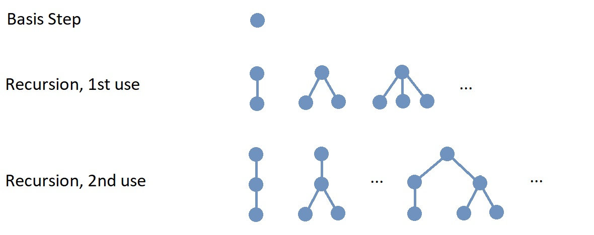
The preceding image shows the basis step and represents, in part, the results of the first and second uses of the recursion step; note that infinitely-many rooted trees are constructed at each use of the recursion step, so we cannot show all the rooted trees produced at any step other than the basis step. Also, we would need to complete infinitely many steps to construct all possible rooted trees, but any one particular rooted tree you want to construct will be produced after only finitely many uses of the recursion step.

7.2.2. Recursively-Defined Functions

A recursively defined function has two parts:

  • Basis Step: Specify the value of the function at zero

  • Recursion Step: Give a rule for finding its value at an integer from its value at smaller integers.

This is similar to a recurrence relation, but using function notation.

Example 9

Consider again the Fibonacci numbers, but this time given by a function \(f(n)\) where \(f(0)=0\), \(f(1)=1\) and \(f(n)=f(n-1)+f(n-2)\) for integers \(n \geq 2.\)

Applying the formula gives \begin{align*} f(2)&=f(1)+f(0)=1+0=1\\ f(3)&=f(2)+f(1)=1+1=2\\ f(4)&=f(3)+f(2)=2+1=3\\ f(5)&=f(4)+f(3)=3+2=5\\ f(6)&=f(5)+f(4)=5+3=8\\ \end{align*} Thinking of this as a recurrence relation we would write \(f_0=0, f_1=1\) and \(f_n=f_{n-1}+f_{n-2}\). Generating the sequence \({0,1,1,2,3,5,8,\ldots}\).

7.3. Solving Recurrence Relations

Recall from earlier in this chapter that a recurrence relation is used to recursively define a sequence of numbers, based on one or more initial conditions, that is, the value(s) of the lowest-indexed term(s).

The phrase "solving a recurrence relation" means finding a closed form that defines the same sequence as the recurrence relation.

Example 10

Solve the recurrence relation \(a_n=a_{n-1}+3\) when \(a_1=2\).

Solution:

We are looking for a closed formula, so we will successively apply the recurrence relation until we see a pattern. \begin{align*} a_2&=a_1+3=2+3\\ a_3&=a_2+3=(2+3)+3 =2+3\cdot 2\\ a_4&=a_3+3=(2+2\cdot 3)+3=2+3\cdot 3\\ \vdots\\ a_n&=a_{n-1}+3=(2+3(n-2))+3=2+3(n-1)\\ \end{align*} So our closed formula is \(a_n=2+3(n-1)\).

You Try

Solve the recurrence relation \(b_n=3b_{n-1}\) when \(a_1=5\).

There are techniques used to solve certain classes of recurrence relations. For now, we will focus on only one case, the class of second-order linear homogeneous recurrence relations.

Example 11 - Solving a second-order linear homogeneous recurrence relation

Consider the recurrence relation \(a_n= b \cdot a_{n-1} + c \cdot a_{n-2}\) where \(b\) and \(c\) are constants and the initial values \(a_0\) and \(a_1\) will be ignored for now.

Notice that you can find at least one solution of the form \(a_n = r^{n}\) for a "suitable" nonzero value of \(r.\) A "suitable" value of \(r\) can be found by stating that you want the following equation to be True for all natural numbers \(n \geq 2\) (and showing that such a "suitable" value of \(r\) actually exists!) \[ r^{n} = b \cdot r^{n-1} + c \cdot r^{n-2} \]

This means that \(r^{2} = b \cdot r^{1} + c \cdot r^{0}\) or more simply \[r^{2} = b \cdot r + c\] and you can solve for \(r\) by factoring or using the quadratic formula.

Notice that if the quadratic equation has two different solutions, then either one of those values can be used as the value of \(r,\) so you’ve actually found two solutions. In fact, you have found all that you need to find every solution, as described in the specific example below.

As an example, consider the recurrence relation \(a_n= 5 \cdot a_{n-1} - 6 \cdot a_{n-2}.\) Based on the previous argument, \(a_n = r^{n}\) is a solution as long as \(r^{2} = 5r - 6,\) that is, \(r^{2} - 5r + 6 = 0.\) The quadratic equation has two solutions: \(r = 2\) ands \(r = 3,\) so each of the closed forms \(a_n = 2^{n}\) and \(a_n = 3^{n}\) describes a solution (but notice that the initial values for \(a_1\) are different.) It is not too difficult to see that any constant multiple of either of the two solutions will give another solution; for example, \(a_n = (-7) \cdot 2^{n}\) and \(a_n = 5 \cdot 3^{n}\) are two more solutions. Also, a sum of any two solutions will still be a solution, so \(a_n = (-7) \cdot 2^{n} + 5 \cdot 3^{n}\) is yet another solution. In fact, we will be able to prove in the chapter on mathematical induction that every solution of this recurrence relation is of the general closed form \(a_n = \alpha \cdot 2^{n} + \beta \cdot 3^{n}\) where \(\alpha\) ("alpha") and \(\beta\) ("beta") are constants, which can be adjusted to match any initial values \(a_0\) and \(a_1\) you want to use: Notice that after substituting 0 for \(n\) you get \(a_0 = \alpha + \beta,\) and after substituting 1 for \(n\) you get \(a_1 = 2 \alpha + 3 \beta,\) so you need to solve a system of two linear equations in two unknowns to determine the values of \(\alpha\) and \(\beta.\)

Note: In the case where the quadratic has only one solution \(r\) (that is, \(r\) is a "double root"), the general closed form solution is \(a_n = (\alpha \cdot n + \beta) \cdot r^{n}\) where \(\alpha\) and \(\beta\) are constants.

You Try

First, find the general closed form solution for the recurrence relation \(b_n=-b_{n-1}+20b_{n-2}.\) Next, find the constants \(\alpha\) and \(\beta\) if the initial conditions \(a_0 =1\) and \(a_1=2\) must also be satisfied.

7.4. Towers Of Hanoi
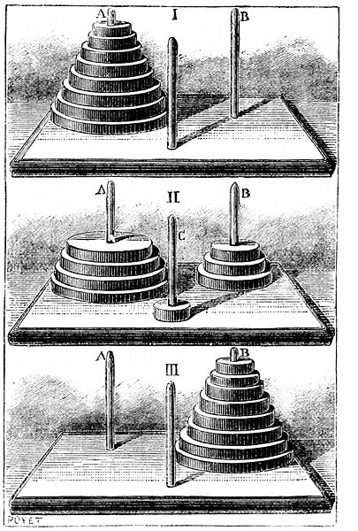
The Tower Of Hanoi

The Towers of Hanoi is a game that was introduced and sold by the French mathematician Édouard Lucas in the 1880s. Lucas stated that the game is "professedly of Indo-Chinese origin" but it seems that Lucas invented this story to market the game.
Image credit: "PSM V26 D464 The tower of hanoi.jpg". This work is in the public domain in its country of origin and other countries and areas where the copyright term is the author’s life plus 70 years or fewer.

At the start of the game, a set of disks of different radii are stacked on a single peg to form a "tower." The disks are stacked so that the radii of the disks decrease as you move up the stack. There are also two empty pegs. The game is won by moving the stack of disks from the original peg to another peg using the following rules

  1. Only one disk can be moved at a time.

  2. The disk at the top of a stack can be moved to the top of another stack or on to an empty peg.

  3. A disk can never be placed on top of a disk that has a smaller radius.

The Towers of Hanoi can be used to explore recursive algorithms, complexity of algorithms, and recurrence relations, based on the following questions.

  • What is the minimal number of moves needed to win the game when there is 1 disk? 2 disks? 3 disks? \(n\) disks?

  • What relationship (if any) is there between the minimal number of moves needed to win an \(n\)-disk game and the minimal number of moves needed to win an \((n-1)\)-disk game?

MORE TO COME!